当前位置：首页>python>Nature期刊图复现 | Python实现多组别多基因表达量柱状散点图

Nature期刊图复现 | Python实现多组别多基因表达量柱状散点图

2026-10-11 05:57:59

来源论文

论文地址：

https://www.nature.com/articles/s41586-023-06249-4

论文题目：

GDF15 promotes weight loss by enhancing energy expenditure in muscle

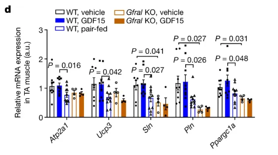
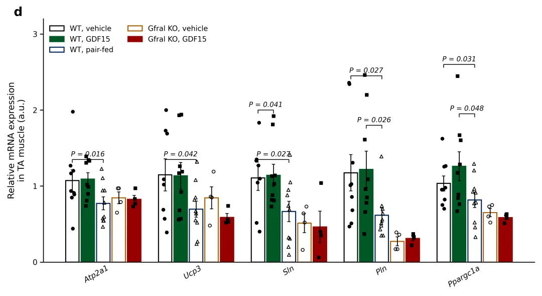
原图释(英)：d, Relative gene expression in muscle. Data are mean ± s.e.m. n = 9 (WT, vehicle; and WT, GDF15), n = 10 (WT, pair-fed) and n = 4 (KO, pair-fed; and KO, GDF15) mice. P values were calculated using two-way ANOVA with Tukey’s multiple-comparison test. a.u., arbitrary units.

原图释(中)：d、肌肉组织中的基因相对表达量。数据以平均值 ± 标准误表示；野生型对照组（溶剂处理）与野生型 GDF15 处理组小鼠样本量n=9，配对饲喂野生型组小鼠n=10，配对饲喂敲除组与敲除 GDF15 处理组小鼠n=4。采用双因素方差分析结合图基多重比较检验计算 P 值；a.u. 为任意单位。

复现图片

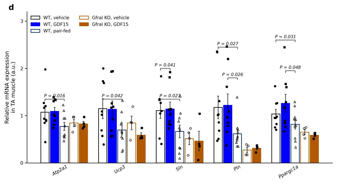
该图通过高分辨率的组合柱状图与散点图，直观展示了不同基因（如Atp2a1、Ucp3等）在五种实验处理条件下的相对mRNA表达水平变化。图中柱体高度及误差棒分别表征各组数据的平均值与标准误（SEM），重叠的独立散点则真实反映了样本检测的个体差异与分布特征。此外，图中所标注的显性 P 值连线精确揭示了组间差异的统计学显著性，为评估不同基因在特定生物学响应或基因敲除背景下的转录表达调控规律提供了严谨、直观的定量科学证据。

配色方案

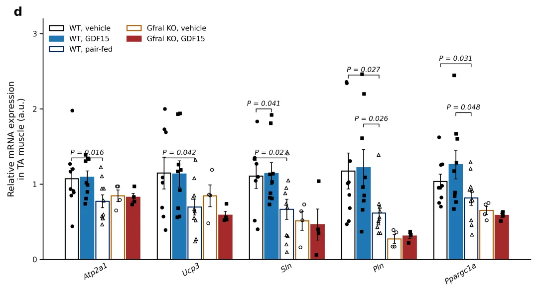
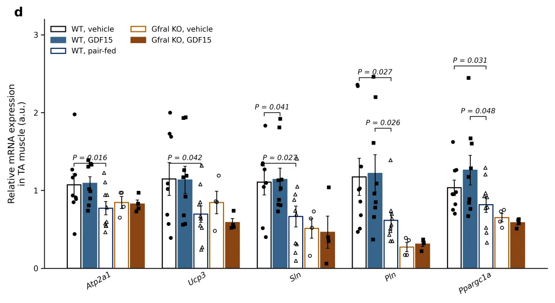
color_schemes = {    1: {'WT, vehicle': 'white', 'WT, GDF15': '#0000ff', 'WT, pair-fed': 'none', 'Gfral KO, vehicle': 'none',        'Gfral KO, GDF15': '#B25900'},  # 方案1: 经典蓝橘高对比科学配色 (Nature/Science 常用)    2: {'WT, vehicle': 'white', 'WT, GDF15': '#1F77B4', 'WT, pair-fed': 'none', 'Gfral KO, vehicle': 'none',        'Gfral KO, GDF15': '#A52A2A'},  # 方案2: 现代学术浅蓝与红褐 (Cell 风格，沉稳不失对比)    3: {'WT, vehicle': 'white', 'WT, GDF15': '#36648B', 'WT, pair-fed': 'none', 'Gfral KO, vehicle': 'none',        'Gfral KO, GDF15': '#8B4513'},  # 方案3: 严谨临床医学灰蓝调 (Lancet 中性冷色调风格)    4: {'WT, vehicle': 'white', 'WT, GDF15': '#005824', 'WT, pair-fed': 'none', 'Gfral KO, vehicle': 'none',        'Gfral KO, GDF15': '#990000'},  # 方案4: 基因组学常用墨绿与暗红 (Nature Genetics 风格)    5: {'WT, vehicle': 'white', 'WT, GDF15': '#3182BD', 'WT, pair-fed': 'none', 'Gfral KO, vehicle': 'none',        'Gfral KO, GDF15': '#E6550D'},  # 方案5: 经典无障碍学术配色 (ColorBrewer 科学明暗配搭)    6: {'WT, vehicle': 'white', 'WT, GDF15': '#08519C', 'WT, pair-fed': 'none', 'Gfral KO, vehicle': 'none',        'Gfral KO, GDF15': '#D94801'},  # 方案6: 细胞生物学亮蓝与暖金 (EMBO Journal 高质感配色)    7: {'WT, vehicle': 'white', 'WT, GDF15': '#0A2240', 'WT, pair-fed': 'none', 'Gfral KO, vehicle': 'none',        'Gfral KO, GDF15': '#CD5C5C'},  # 方案7: 跨学科深邃蓝与珊瑚红 (Science 封面高频色彩)    8: {'WT, vehicle': 'white', 'WT, GDF15': '#4A148C', 'WT, pair-fed': 'none', 'Gfral KO, vehicle': 'none',        'Gfral KO, GDF15': '#8D6E63'},  # 方案8: 神经科学冷紫与赭石 (Nature Neuroscience 风格)    9: {'WT, vehicle': 'white', 'WT, GDF15': '#004D40', 'WT, pair-fed': 'none', 'Gfral KO, vehicle': 'none',        'Gfral KO, GDF15': '#BF360C'},  # 方案9: 传统学术暗青与锈红 (生理与药理学经典经典)    10: {'WT, vehicle': 'white', 'WT, GDF15': '#1A237E', 'WT, pair-fed': 'none', 'Gfral KO, vehicle': 'none',         'Gfral KO, GDF15': '#AD1457'},  # 方案10: 现代神经科学深靛蓝与玫瑰金 (高雅前沿感)    11: {'WT, vehicle': 'white', 'WT, GDF15': '#1B5E20', 'WT, pair-fed': 'none', 'Gfral KO, vehicle': 'none',         'Gfral KO, GDF15': '#455A64'},  # 方案11: 环境科学森林绿与矿物灰 (Nature Climate Change)    12: {'WT, vehicle': 'white', 'WT, GDF15': '#0D47A1', 'WT, pair-fed': 'none', 'Gfral KO, vehicle': 'none',         'Gfral KO, GDF15': '#E65100'},  # 方案12: 生物信息海军蓝与明艳橙 (兼顾黑白打印明暗度)    13: {'WT, vehicle': 'white', 'WT, GDF15': '#01579B', 'WT, pair-fed': 'none', 'Gfral KO, vehicle': 'none',         'Gfral KO, GDF15': '#A0522D'},  # 方案13: 自然科学泥土黄与深海蓝 (地球科学经典对比)    14: {'WT, vehicle': 'white', 'WT, GDF15': '#311B92', 'WT, pair-fed': 'none', 'Gfral KO, vehicle': 'none',         'Gfral KO, GDF15': '#556B2F'},  # 方案14: 综合科学暗紫与橄榄绿 (PNAS 常见非对称对比色)    15: {'WT, vehicle': 'white', 'WT, GDF15': '#880E4F', 'WT, pair-fed': 'none', 'Gfral KO, vehicle': 'none',         'Gfral KO, GDF15': '#37474F'},  # 方案15: 临床免疫学暗红与深灰 (Blood 期刊常用沉稳色)    16: {'WT, vehicle': 'white', 'WT, GDF15': '#004B49', 'WT, pair-fed': 'none', 'Gfral KO, vehicle': 'none',         'Gfral KO, GDF15': '#5D4037'},  # 方案16: 结构生物学宝石绿与巧克力色 (适合结构晶体数据)    17: {'WT, vehicle': 'white', 'WT, GDF15': '#2C3E50', 'WT, pair-fed': 'none', 'Gfral KO, vehicle': 'none',         'Gfral KO, GDF15': '#D35400'},  # 方案17: 生物材料学石板蓝与落叶橙 (JACS 论文常用优雅色)    18: {'WT, vehicle': 'white', 'WT, GDF15': '#0072B2', 'WT, pair-fed': 'none', 'Gfral KO, vehicle': 'none',         'Gfral KO, GDF15': '#D55E00'},  # 方案18: 经典色弱友好型冷暖色系 (国际学界无障碍评审标准)    19: {'WT, vehicle': 'white', 'WT, GDF15': '#006064', 'WT, pair-fed': 'none', 'Gfral KO, vehicle': 'none',         'Gfral KO, GDF15': '#263238'},  # 方案19: 尖端生物技术量子灰与极光青 (Nature Biotech 风格)    20: {'WT, vehicle': 'white', 'WT, GDF15': '#4A0E17', 'WT, pair-fed': 'none', 'Gfral KO, vehicle': 'none',         'Gfral KO, GDF15': '#0A192F'}  # 方案20: 微生物学经典勃艮第红与午夜蓝 (冷暖交替对比)}

完整代码

import osimport numpy as npimport pandas as pdimport matplotlib.pyplot as plt# 1. 基础配置与创建输出文件夹output_dir = "图表"if not os.path.exists(output_dir):    os.makedirs(output_dir)excel_file = "data.xlsx"if not os.path.exists(excel_file):    raise FileNotFoundError(f"未在当前目录下找到 {excel_file} 文件，请检查文件名和路径。")# 定义展示的基因顺序target_genes = ['Atp2a1', 'Ucp3', 'Sln', 'Pln', 'Ppargc1a']# 定义图表展示的标准组名顺序conditions_order = ['WT, vehicle', 'WT, GDF15', 'WT, pair-fed', 'Gfral KO, vehicle', 'Gfral KO, GDF15']# 2. 20种配色方案字典color_schemes = {    1: {'WT, vehicle': 'white', 'WT, GDF15': '#0000ff', 'WT, pair-fed': 'none', 'Gfral KO, vehicle': 'none',        'Gfral KO, GDF15': '#B25900'},  # 方案1: 经典蓝橘高对比科学配色 (Nature/Science 常用)}# 选择第 1 种配色方案selected_scheme = 1bar_colors = color_schemes[selected_scheme]# 3. 动态配置柱子外边框颜色edge_colors = {cond: ('black' if color == 'white' else color) for cond, color in bar_colors.items()}for cond in edge_colors:    if edge_colors[cond] == 'none':        edge_colors[cond] = '#002060' if 'WT' in cond else '#B25900'# 散点风格配置（统一为纯黑色散点）scatter_styles = {    'WT, vehicle': {'marker': 'o', 'color': 'black', 's': 20, 'zorder': 4},    'WT, GDF15': {'marker': 's', 'color': 'black', 's': 18, 'zorder': 4},    'WT, pair-fed': {'marker': '^', 'color': 'black', 's': 22, 'facecolors': 'none', 'linewidths': 1, 'zorder': 4},    'Gfral KO, vehicle': {'marker': 'o', 'color': 'black', 's': 20, 'facecolors': 'none', 'linewidths': 1, 'zorder': 4},    'Gfral KO, GDF15': {'marker': 's', 'color': 'black', 's': 18, 'zorder': 4}}# 4. 初始化数据结构plot_data = {gene: {cond: {'mean': 0, 'sem': 0, 'values': []} for cond in conditions_order} for gene in target_genes}# 打开 Excel 文件，获取所有 Sheet 的名字列表xl = pd.ExcelFile(excel_file)sheet_names = xl.sheet_namesif len(sheet_names) < 5:    raise ValueError(f"Excel 文件中的 Sheet 数量不足 5 个，当前只有 {len(sheet_names)} 个。")# 5. 按照物理顺序依次读取 Sheet 并处理数据for idx, cond in enumerate(conditions_order):    actual_sheet_name = sheet_names[idx]    df_sheet = pd.read_excel(excel_file, sheet_name=actual_sheet_name, header=None)    sheet_first_col = df_sheet.iloc[:, 0].astype(str).str.strip().tolist()    sheet_first_col_lower = [x.lower() for x in sheet_first_col]    for gene in target_genes:        gene_lower = gene.lower()        if gene_lower in sheet_first_col_lower:            row_idx = sheet_first_col_lower.index(gene_lower)            row_values = df_sheet.iloc[row_idx, 1:]            sample_values = pd.to_numeric(row_values, errors='coerce').dropna().values            plot_data[gene][cond]['values'] = sample_values.tolist()        else:            print(f"提示: 在第 {idx + 1} 个 Sheet [{actual_sheet_name}] 中未找到基因: {gene}")# 计算均值和标准误 (SEM)for gene in target_genes:    for cond in conditions_order:        vals = np.array(plot_data[gene][cond]['values'])        if len(vals) > 0:            plot_data[gene][cond]['mean'] = np.mean(vals)            plot_data[gene][cond]['sem'] = np.std(vals, ddof=1) / np.sqrt(len(vals)) if len(vals) > 1 else 0# 6. 开始绘制高精仿科研图表fig, ax = plt.subplots(figsize=(11, 6), dpi=300)n_genes = len(target_genes)n_conds = len(conditions_order)bar_width = 0.13gap = 0.02group_width = n_conds * (bar_width + gap) + 0.15pos_base = np.arange(n_genes) * group_widthlegend_handles = []for idx, cond in enumerate(conditions_order):    x_positions = pos_base + idx * (bar_width + gap)    means = [plot_data[gene][cond]['mean'] for gene in target_genes]    sems = [plot_data[gene][cond]['sem'] for gene in target_genes]    bars = ax.bar(x_positions, means, width=bar_width,                  color=bar_colors[cond], edgecolor=edge_colors[cond], linewidth=1.5,                  yerr=sems, capsize=2.5, error_kw={'ecolor': 'black', 'elinewidth': 1.2},                  zorder=2)    legend_handles.append(bars[0])    for g_idx, gene in enumerate(target_genes):        vals = plot_data[gene][cond]['values']        if len(vals) > 0:            np.random.seed(42 + idx)            jitter = np.random.uniform(-0.02, 0.02, len(vals))            ax.scatter([x_positions[g_idx]] * len(vals) + jitter, vals, **scatter_styles[cond])# 7. 图表细节美化与坐标轴规范ax.set_ylabel('Relative mRNA expression\nin TA muscle (a.u.)', fontsize=13, labelpad=10)ax.set_xticks(pos_base + (n_conds * (bar_width + gap) - gap) / 2)ax.set_xticklabels(target_genes, rotation=30, ha='right', fontsize=12, fontweight='normal', style='italic')ax.set_ylim(0, 3.2)ax.set_yticks([0, 1, 2, 3])ax.tick_params(axis='both', which='major', labelsize=11, direction='out', length=5, width=1.2)ax.tick_params(axis='x', length=0)ax.spines['top'].set_visible(False)ax.spines['right'].set_visible(False)ax.spines['left'].set_linewidth(1.2)ax.spines['bottom'].set_linewidth(1.2)ax.grid(False)ax.legend(legend_handles, conditions_order, loc='upper left', frameon=False, ncol=2, fontsize=10.5)# 在图表左上角添加加粗的序号 "d"ax.text(-0.06, 1.05, 'd', transform=ax.transAxes, fontsize=18, fontweight='bold', va='top', ha='left')# 8. 标注原图中的显著性 P 值连线def add_p_value(gene_name, c1_idx, c2_idx, p_str, y_base, tick_h=0.04):    g_idx = target_genes.index(gene_name)    x1 = pos_base[g_idx] + c1_idx * (bar_width + gap)    x2 = pos_base[g_idx] + c2_idx * (bar_width + gap)    ax.plot([x1, x1, x2, x2], [y_base - tick_h, y_base, y_base, y_base - tick_h], color='black', lw=1)    ax.text((x1 + x2) / 2, y_base + 0.02, p_str, ha='center', va='bottom', fontsize=10, style='italic')add_p_value('Atp2a1', 0, 2, 'P = 0.016', 1.35)add_p_value('Ucp3', 0, 2, 'P = 0.042', 1.35)add_p_value('Sln', 0, 2, 'P = 0.027', 1.35)add_p_value('Sln', 0, 1, 'P = 0.041', 2.00)add_p_value('Pln', 1, 2, 'P = 0.026', 1.80)add_p_value('Pln', 0, 2, 'P = 0.027', 2.45)add_p_value('Ppargc1a', 1, 2, 'P = 0.048', 1.95)add_p_value('Ppargc1a', 0, 2, 'P = 0.031', 2.60)# 9. 保存高清图片output_path = os.path.join(output_dir, "TA_muscle_mRNA_expression_exact.png")plt.tight_layout()plt.savefig(output_path, dpi=300)plt.close()print(f"图表已成功处理完毕并保存至: {output_path}")