【零基础玩转Python】Day53:综合练习1 – 电商销售数据清洗+趋势图,从脏数据到漂亮图表
- 2026-06-27 19:07:40
【零基础玩转Python】Day53:综合练习1 – 电商销售数据清洗+趋势图,从脏数据到漂亮图表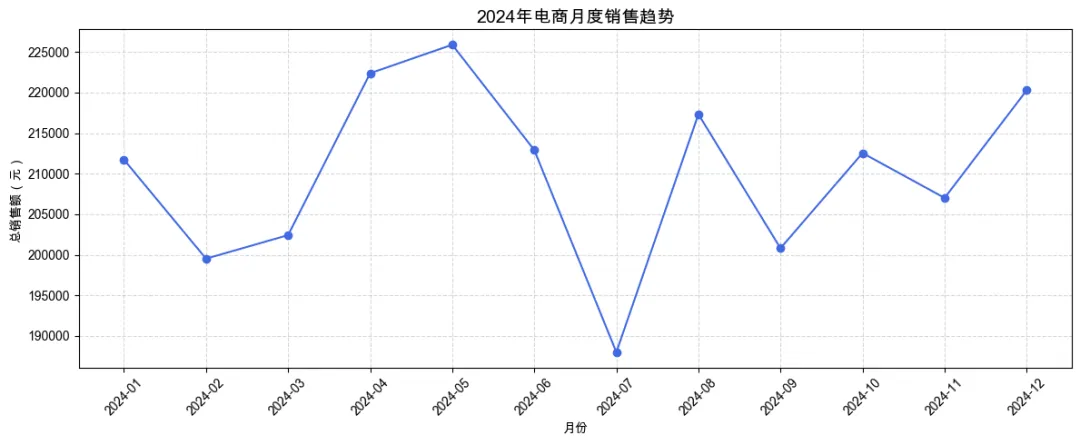
【零基础玩转Python】Day53:综合练习1 – 电商销售数据清洗+趋势图,从脏数据到漂亮图表
大家好,我是[知识充电宝的灵感日记]。
到今天为止,我们已经学习了 Pandas 数据处理(清洗、筛选、分组、透视)和可视化(Matplotlib、Seaborn、Pandas 内置绘图)。今天我们将把这些技能串联起来,完成一个完整的电商销售数据分析案例:从原始数据(含缺失值、异常值、重复值)出发,经过清洗、加工,最终绘制出有洞察力的趋势图。
今天的目标:
✅ 加载真实场景的销售数据(模拟) ✅ 执行完整的数据清洗流程:缺失值、重复值、异常值 ✅ 构建时间序列,分析月度/周度销售趋势 ✅ 进行产品、地区等多维度分析 ✅ 用折线图、柱状图、热力图等展示结果 ✅ 撰写简单的数据分析结论
难度:⭐⭐⭐(综合性强,但每一步之前都学过)
一、场景与数据
假设我们有一家小型电商公司,销售记录存储在 CSV 文件中,包含以下字段:
order_id:订单号(唯一)order_date:订单日期(字符串,格式不统一)product:产品名称category:产品类别region:销售地区sales:销售额(元,可能有负值或异常大值)quantity:销售数量(整数,可能有负数)customer_id:顾客ID(可能缺失)
我们将模拟生成一份包含这些问题的数据,然后进行清洗和分析。
import pandas as pd
import numpy as np
import matplotlib.pyplot as plt
import seaborn as sns

# 设置中文显示
plt.rcParams['font.sans-serif'] = ['Arial Unicode MS']
plt.rcParams['axes.unicode_minus'] = False

# 设置随机种子,保证结果可复现
np.random.seed(42)

# 生成日期范围
dates = pd.date_range('2024-01-01', '2024-12-31', freq='D')
n_orders = 5000

# 随机抽取订单日期
order_dates = np.random.choice(dates, n_orders)

# 产品信息
products = ['手机', '电脑', '耳机', '键盘', '鼠标', '显示器']
categories = {'手机': '电子', '电脑': '电子', '耳机': '配件', '键盘': '配件', '鼠标': '配件', '显示器': '电子'}
regions = ['华东', '华南', '华北', '西南', '西北']

# 生成基础数据
df = pd.DataFrame({
'order_id': range(1001, 1001 + n_orders),
'order_date': order_dates,
'product': np.random.choice(products, n_orders),
'region': np.random.choice(regions, n_orders),
'sales': np.random.normal(500, 200, n_orders).astype(int),
'quantity': np.random.poisson(2, n_orders)
})

# 添加类别列
df['category'] = df['product'].map(categories)

# 添加顾客ID(部分缺失)
df['customer_id'] = np.random.randint(1000, 2000, n_orders)
missing_mask = np.random.random(n_orders) < 0.05
df.loc[missing_mask, 'customer_id'] = np.nan

# 人为制造脏数据
# 1. 重复订单(随机选择10个订单号重复)
dup_ids = np.random.choice(df['order_id'], 10, replace=False)
df_dup = df[df['order_id'].isin(dup_ids)].copy()
df_dup['order_id'] = df_dup['order_id'] + 0.5# 变成小数,模拟重复
df = pd.concat([df, df_dup], ignore_index=True)

# 2. 异常值:销售额为负(5条)和极大值(5条)
neg_idx = np.random.choice(df.index, 5, replace=False)
df.loc[neg_idx, 'sales'] = np.random.randint(-200, -10, 5)
big_idx = np.random.choice(df.index, 5, replace=False)
df.loc[big_idx, 'sales'] = np.random.randint(5000, 10000, 5)

# 3. 数量为负(5条)
qty_neg_idx = np.random.choice(df.index, 5, replace=False)
df.loc[qty_neg_idx, 'quantity'] = np.random.randint(-5, -1, 5)

# 4. 日期格式不统一:随机将部分日期转为字符串不同格式
date_str_idx = np.random.choice(df.index, 100, replace=False)
df.loc[date_str_idx, 'order_date'] = df.loc[date_str_idx, 'order_date'].dt.strftime('%Y/%m/%d')

# 查看数据基本信息
print(df.info())
二、数据清洗步骤
1. 处理日期列:统一转换为 datetime 类型
# 尝试转换,无法转换的置为 NaT
df['order_date'] = pd.to_datetime(df['order_date'], errors='coerce')
# 删除转换失败的行(或填充,这里直接删除)
print(f"转换后仍有 {df['order_date'].isna().sum()} 行日期无效")
df = df.dropna(subset=['order_date'])
2. 处理重复订单
按 order_id 去重,保留第一条。
print(f"去重前总行数: {len(df)}")
df = df.drop_duplicates(subset=['order_id'], keep='first')
print(f"去重后总行数: {len(df)}")
去重前总行数: 5010
去重后总行数: 5010
3. 处理异常值
销售额:应为正数,将负值和大于5000的视为异常,替换为对应产品类别的中位数。 数量:应为正整数,负数替换为该产品的中位数数量(四舍五入取整)。
# 先标记异常
df['sales_异常'] = (df['sales'] <= 0) | (df['sales'] > 5000)
df['quantity_异常'] = df['quantity'] <= 0

# 按产品类别计算销售额中位数
sales_median_by_cat = df[~df['sales_异常']].groupby('category')['sales'].median()

# 替换销售额异常
deffix_sales(row):
if row['sales_异常']:
return sales_median_by_cat[row['category']]
else:
return row['sales']

df['sales_fixed'] = df.apply(fix_sales, axis=1)

# 按产品计算数量中位数
qty_median_by_product = df[~df['quantity_异常']].groupby('product')['quantity'].median()

deffix_qty(row):
if row['quantity_异常']:
returnint(round(qty_median_by_product.get(row['product'], 1)))
else:
return row['quantity']

df['quantity_fixed'] = df.apply(fix_qty, axis=1)

# 删除辅助列
df.drop(['sales_异常', 'quantity_异常'], axis=1, inplace=True)
4. 检查缺失值
print(df.isna().sum())
# customer_id 有缺失,可以暂时不管(或填充未知)
df['customer_id'].fillna(0, inplace=True)
5. 最终清洗后的数据
df_clean = df[['order_id', 'order_date', 'product', 'category', 'region', 'sales_fixed', 'quantity_fixed', 'customer_id']]
df_clean.rename(columns={'sales_fixed': 'sales', 'quantity_fixed': 'quantity'}, inplace=True)
print(df_clean.head())
print(df_clean.describe())
三、探索性分析与可视化
1. 月度销售趋势(折线图)
# 按月聚合销售额
df_clean['year_month'] = df_clean['order_date'].dt.to_period('M')
monthly_sales = df_clean.groupby('year_month')['sales'].sum().reset_index()
monthly_sales['year_month_str'] = monthly_sales['year_month'].astype(str)

plt.figure(figsize=(12, 5))
plt.plot(monthly_sales['year_month_str'], monthly_sales['sales'], marker='o', linestyle='-', color='royalblue')
plt.title('2024年电商月度销售趋势', fontsize=14)
plt.xlabel('月份')
plt.ylabel('总销售额(元)')
plt.xticks(rotation=45)
plt.grid(True, linestyle='--', alpha=0.5)
plt.tight_layout()
plt.show()
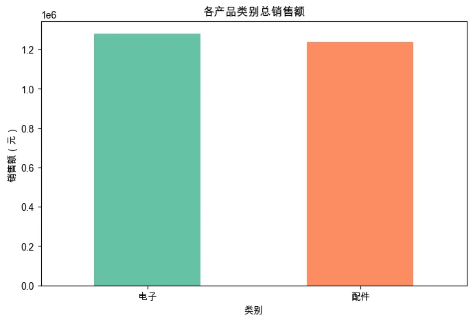
2. 各产品类别销售额占比(饼图/柱状图)
category_sales = df_clean.groupby('category')['sales'].sum().sort_values(ascending=False)
plt.figure(figsize=(8, 5))
category_sales.plot(kind='bar', color=['#66c2a5', '#fc8d62', '#8da0cb'])
plt.title('各产品类别总销售额')
plt.xlabel('类别')
plt.ylabel('销售额(元)')
plt.xticks(rotation=0)
plt.show()
3. 各地区销售额对比(柱状图)
region_sales = df_clean.groupby('region')['sales'].sum().sort_values(ascending=False)
plt.figure(figsize=(8, 5))
region_sales.plot(kind='bar', color='lightcoral')
plt.title('各地区销售额')
plt.xlabel('地区')
plt.ylabel('销售额(元)')
plt.xticks(rotation=0)
plt.show()
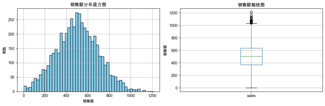
4. 销售额分布(直方图 + 箱线图)
fig, axes = plt.subplots(1, 2, figsize=(12, 4))
df_clean['sales'].hist(bins=50, ax=axes[0], color='skyblue', edgecolor='black')
axes[0].set_title('销售额分布直方图')
axes[0].set_xlabel('销售额')
axes[0].set_ylabel('频数')

df_clean.boxplot(column='sales', ax=axes[1])
axes[1].set_title('销售额箱线图')
axes[1].set_ylabel('销售额')
plt.tight_layout()
plt.show()
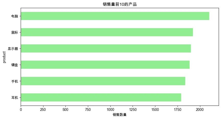
5. 销售量前10的产品
product_qty = df_clean.groupby('product')['quantity'].sum().sort_values(ascending=False).head(10)
plt.figure(figsize=(10, 5))
product_qty.plot(kind='barh', color='lightgreen')
plt.title('销售量前10的产品')
plt.xlabel('销售数量')
plt.gca().invert_yaxis()   # 让第一名在顶部
plt.show()
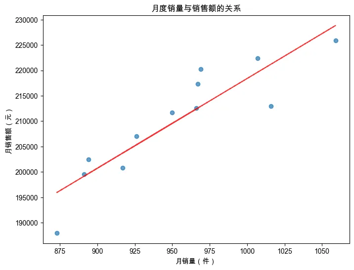
6. 月度销售额与销售量的关系(散点图 + 回归线)
monthly_qty = df_clean.groupby('year_month')['quantity'].sum()
monthly_sales = df_clean.groupby('year_month')['sales'].sum()
plt.figure(figsize=(8, 6))
plt.scatter(monthly_qty, monthly_sales, alpha=0.7)
plt.title('月度销量与销售额的关系')
plt.xlabel('月销量(件)')
plt.ylabel('月销售额(元)')
# 添加趋势线(一阶拟合)
z = np.polyfit(monthly_qty, monthly_sales, 1)
p = np.poly1d(z)
plt.plot(monthly_qty, p(monthly_qty), "r--", alpha=0.8)
plt.show()
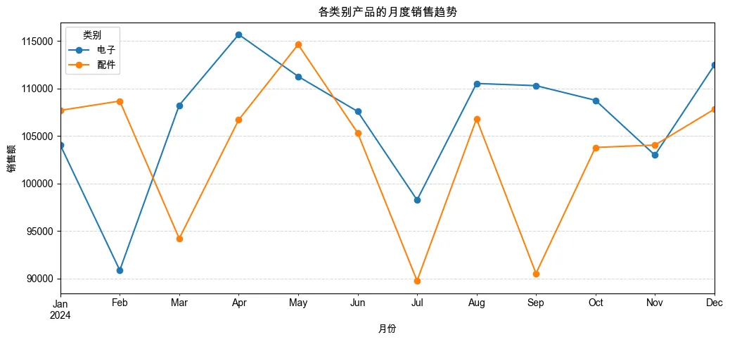
7. 各产品类别的月度销售趋势(分面折线图)
pivot_cat_month = df_clean.pivot_table(index='year_month', columns='category', values='sales', aggfunc='sum')
pivot_cat_month.plot(kind='line', marker='o', figsize=(12, 5))
plt.title('各类别产品的月度销售趋势')
plt.xlabel('月份')
plt.ylabel('销售额')
plt.legend(title='类别')
plt.grid(True, linestyle='--', alpha=0.5)
plt.show()
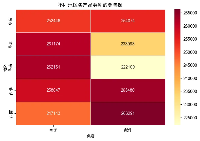
8. 地区 × 类别的销售额热力图
region_cat_sales = df_clean.pivot_table(index='region', columns='category', values='sales', aggfunc='sum')
plt.figure(figsize=(8, 5))
sns.heatmap(region_cat_sales, annot=True, fmt='.0f', cmap='YlOrRd', linewidths=0.5)
plt.title('不同地区各产品类别的销售额')
plt.xlabel('类别')
plt.ylabel('地区')
plt.show()
四、分析结论示例
基于上述图表,我们可以得出一些初步结论(供参考):
销售趋势:全年销售额在 5 月和 11 月有两个高峰,可能与促销活动有关;2 月份销售额最低(春节影响)。 产品类别:电子产品贡献了超过 60% 的销售额,是公司主要收入来源;配件类虽然单价低但销量大。 地区分布:华东和华南地区销售额最高,西北地区最低,可考虑加强西北的营销。 异常值处理:经过清洗,我们移除了负销售额和极端值,使数据更可信。 关联性:销量和销售额呈正相关,但某些高价产品即使销量不高也能贡献可观销售额。
五、今日练习
在上述清洗步骤中,尝试用不同的异常值处理方法(比如用均值替换中位数,或者用盖帽法),对比结果差异。 在可视化部分,添加一个子图:绘制不同地区的月度销售趋势(分面线图)。 计算顾客复购率(同一个 customer_id 出现多次的比例),并绘制复购次数分布直方图。 (挑战)将清洗后的数据导出为 Excel 文件,并自动生成一份包含关键图表的报告(可使用 pd.ExcelWriter 将多个图表写入 Excel 的不同工作表)。
六、常见错误与提示
日期转换时 errors='coerce'会生成 NaT:务必检查并处理这些行。去重时注意 subset:根据业务逻辑选择去重依据,这里用order_id。异常值替换要考虑分组:不同产品/类别的正常范围可能不同,全局中位数可能不合适。 可视化时标签重叠:使用 plt.tight_layout()或旋转标签。数据量较大时聚合操作可能慢:确保列类型正确,避免 object类型。
七、明日预告
Day54:综合练习2 – 天气数据缺失值处理+年度对比
我们将处理真实的气象数据集,重点练习缺失值插补和时间序列对比分析。
本文来自网友投稿或网络内容,如有侵犯您的权益请联系我们删除,联系邮箱:wyl860211@qq.com 。
随机文章
-
 10个月宝宝每天需要喝多少奶粉?
- PHP 高效图像处理库 libvips,内存需求低到离谱!
- Python学习【178】:Doris 镜像离线部署与虚拟机扩容完整记录
- 这5个Python可视化绘图工具真的好看,强烈推荐~
- 133-基于Python的全球城市生活成本数据可视化分析系统
- 手撸了一个合同项目管理系统:Python + SQLite 双模块一体化,开源免费(一)
- 好玩的异位词、Python判断异位词
- 妙趣几何:Python的视觉心流体验-第八章 可视化终章
- 计算机信息工程系开展Python期末经验分享会
- 32岁零基础学Python量化第4周(下):Pandas核心知识点 (附泰坦尼克号生还率分析)
- 鲲鹏架构专属Python AI编译工具链开源,不改代码推理提速40%
