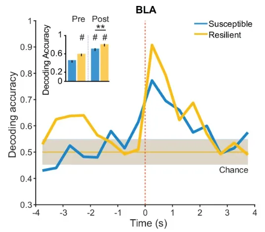
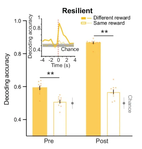
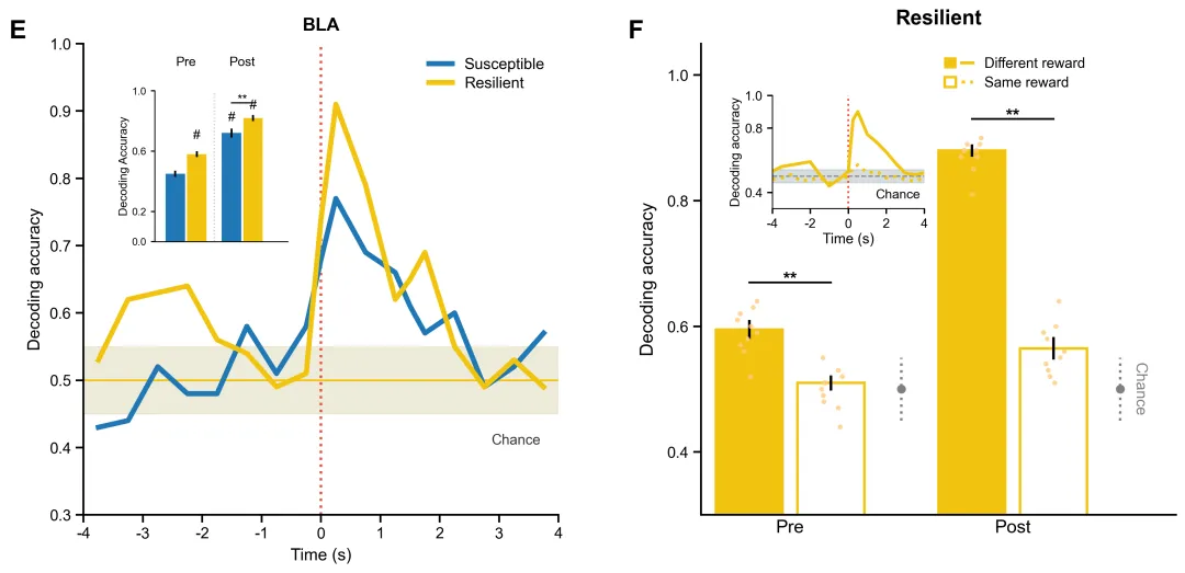
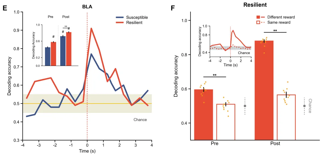
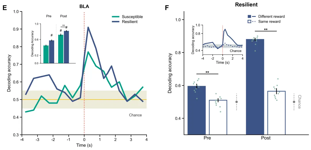
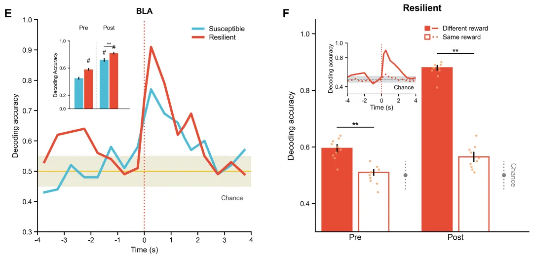
import osimport matplotlib.pyplot as pltimport matplotlib.patches as mpatchesimport matplotlib.lines as mlinesfrom matplotlib.legend_handler import HandlerTupleimport numpy as npimport pandas as pd# ==========================================# 1. 自动创建图表文件夹并读取数据# ==========================================output_dir = "图表"if not os.path.exists(output_dir): os.makedirs(output_dir)excel_file1 = "data.xlsx"excel_file2 = "data2.xlsx"if not os.path.exists(excel_file1) or not os.path.exists(excel_file2): raise FileNotFoundError("请确保 data.xlsx 和 data2.xlsx 数据文件均存在于当前目录下!")df_main_E = pd.read_excel(excel_file1, sheet_name="Main_Line_Data")df_inset_E = pd.read_excel(excel_file1, sheet_name="Inset_Bar_Data")df_bar_F = pd.read_excel(excel_file2, sheet_name="Main_Bar_Data")df_scatter_F = pd.read_excel(excel_file2, sheet_name="Scatter_Points_Data")df_inset_F = pd.read_excel(excel_file2, sheet_name="Inset_Line_Data")# ==========================================# 2. 学术期刊专业科研配色方案字典 (20种)# ==========================================color_palettes = { 1: {"sus": "#1f77b4", "res": "#f1c40f", "scatter": "#ffcc80"}, # 方案1: 经典 Nature 神经科学风格 (经典蓝 + 活力金黄 + 柔和浅橙散点) 2: {"sus": "#3c5488", "res": "#e64b35", "scatter": "#f39c12"}, # 方案2: Lancet 柳叶刀风格 (海军蓝 + 经典朱红 + 样本暖橙) 3: {"sus": "#00a087", "res": "#3c5488", "scatter": "#79af97"}, # 方案3: NEJM 新英格兰医学风格 (薄荷绿 + 深邃海蓝 + 淡绿散点) 4: {"sus": "#4dbbd5", "res": "#e64b35", "scatter": "#f4a261"}, # 方案4: JAMA 美国医学会风格 (天空蓝 + 艳丽珊瑚红 + 浅珊瑚散点) 5: {"sus": "#1f77b4", "res": "#ff7f0e", "scatter": "#ffbb78"}, # 方案5: Science 科学通用折线柱状图对比色 (标准蓝 + 亮橙 + 柔和浅红) 6: {"sus": "#2ca02c", "res": "#d62728", "scatter": "#ff9896"}, # 方案6: Cell 细胞生理与发育生物学常规色 (植物绿 + 细胞红 + 浅粉散点) 7: {"sus": "#9467bd", "res": "#8c564b", "scatter": "#c49c94"}, # 方案7: Nature Genetics 遗传学基因图谱常用色 (高贵紫 + 泥土棕 + 浅褐散点) 8: {"sus": "#e377c2", "res": "#7f7f7f", "scatter": "#c7c7c7"}, # 方案8: Nature Communication 综合期刊对比色 (亮粉紫 + 中性灰 + 浅灰散点) 9: {"sus": "#17beccf0", "res": "#bcbd22f0", "scatter": "#dbdb8d"}, # 方案9: IEEE 电子与计算科学高对比高饱和度色 (青翠蓝 + 芥末黄 + 淡黄散点) 10: {"sus": "#4a148c", "res": "#00695c", "scatter": "#80cbc4"}, # 方案10: Material Today 材料及物理科学冷色调 (深紫罗兰 + 墨绿 + 湖绿散点) 11: {"sus": "#20b2aa", "res": "#ff6347", "scatter": "#ffa07a"}, # 方案11: BioMed Central 生物医药高亮醒目对比色 (浅海蓝 + 番茄红 + 肉粉散点) 12: {"sus": "#2f4f4f", "res": "#d2691e", "scatter": "#f4a460"}, # 方案12: Ecology 传统生态与环境科学配色 (暗石板灰 + 巧克力棕 + 沙滩黄散点) 13: {"sus": "#002060", "res": "#ed7d31", "scatter": "#f8cbad"}, # 方案13: Clinical Chemistry 临床化学高端严谨色 (经典藏青 + 现代橙 + 浅肤色散点) 14: {"sus": "#5b9bd5", "res": "#70ad47", "scatter": "#c5e0b4"}, # 方案14: Frontiers 边界系列期刊高频商务质感色 (柔和钢蓝 + 橄榄绿 + 浅绿散点) 15: {"sus": "#3a86ff", "res": "#ff006e", "scatter": "#ffbe0b"}, # 方案15: Advanced Materials 顶刊高现代感色彩 (电光蓝 + 荧光粉红 + 明黄散点) 16: {"sus": "#03045e", "res": "#00b4d8", "scatter": "#caf0f8"}, # 方案16: Nature Climate Change 气候环境渐变层次色 (极地深蓝 + 冰川蓝 + 极浅蓝散点) 17: {"sus": "#6d597a", "res": "#e56b6f", "scatter": "#eaac8b"}, # 方案17: Social Science 社会学与群体行为学高级暗色 (莫兰迪紫 + 砖红 + 浅杏散点) 18: {"sus": "#4361ee", "res": "#4cc9f0", "scatter": "#b5e2fa"}, # 方案18: BioInformatics 生物信息学数字化高显色 (科技蓝 + 亮青色 + 淡蓝散点) 19: {"sus": "#264653", "res": "#e76f51", "scatter": "#f4a261"}, # 方案19: Earth Science 地球科学地质构造色 (深海青 + 铁锈红 + 黄土散点) 20: {"sus": "#2b2d42", "res": "#d90429", "scatter": "#ef233c"} # 方案20: Oncogene 肿瘤学癌细胞浸润高警示色 (黑金属灰 + 警示深红 + 鲜红散点)}# 选择方案 1selected_palette = color_palettes[1]color_sus = selected_palette["sus"]color_res = selected_palette["res"]color_main_F = selected_palette["res"]color_edge_F = selected_palette["res"]color_scatter_F = selected_palette["scatter"]# ==========================================# 3. 设置全局绘图样式# ==========================================plt.rcParams["font.family"] = "sans-serif"plt.rcParams["font.sans-serif"] = ["Arial", "Liberation Sans", "DejaVu Sans"]plt.rcParams["axes.unicode_minus"] = Falsefig, (ax_E, ax_F) = plt.subplots(1, 2, figsize=(13.5, 6.5))fig.subplots_adjust(left=0.08, right=0.95, top=0.90, bottom=0.12, wspace=0.3)# ==========================================# 4. 绘制左侧【图 E】# ==========================================ax_E.axhspan(0.45, 0.55, color="#e4dec2", alpha=0.6, zorder=1)ax_E.axhline(0.5, color="#f1c40f", linestyle="-", linewidth=1.5, zorder=2)ax_E.text(3.7, 0.42, "Chance", fontsize=11, color="#333333", ha="right", va="top")ax_E.axvline(0, color="#e74c3c", linestyle=":", linewidth=2, zorder=2)ax_E.text(0, 1.02, "BLA", fontsize=14, fontweight="bold", color="black", ha="center", va="bottom", transform=ax_E.get_xaxis_transform())ax_E.plot(df_main_E["Time"], df_main_E["Susceptible"], color=color_sus, linewidth=4, label="Susceptible", zorder=3)ax_E.plot(df_main_E["Time"], df_main_E["Resilient"], color=color_res, linewidth=4, label="Resilient", zorder=4)ax_E.set_xlabel("Time (s)", fontsize=13, labelpad=5)ax_E.set_ylabel("Decoding accuracy", fontsize=13, labelpad=5)ax_E.set_xlim(-4, 4)ax_E.set_ylim(0.3, 1.0)ax_E.set_xticks(range(-4, 5))ax_E.set_yticks(np.arange(0.3, 1.1, 0.1))ax_E.tick_params(axis="both", which="major", labelsize=12, width=1.5, length=6)ax_E.spines["top"].set_visible(False)ax_E.spines["right"].set_visible(False)ax_E.spines["left"].set_linewidth(1.5)ax_E.spines["bottom"].set_linewidth(1.5)ax_E.legend(loc="upper right", frameon=False, fontsize=12, handlelength=1.5, labelspacing=0.3)ax_E.text(-0.12, 1.05, "E", transform=ax_E.transAxes, fontsize=20, fontweight="bold", va="top", ha="right")ax_inset_E = ax_E.inset_axes([0.15, 0.58, 0.28, 0.32])pre_sus = df_inset_E[(df_inset_E["Phase"] == "Pre") & (df_inset_E["Group"] == "Susceptible")].iloc[0]pre_res = df_inset_E[(df_inset_E["Phase"] == "Pre") & (df_inset_E["Group"] == "Resilient")].iloc[0]post_sus = df_inset_E[(df_inset_E["Phase"] == "Post") & (df_inset_E["Group"] == "Susceptible")].iloc[0]post_res = df_inset_E[(df_inset_E["Phase"] == "Post") & (df_inset_E["Group"] == "Resilient")].iloc[0]bar_width_E = 0.38x_pre_sus = 1.0x_pre_res = 1.0 + bar_width_E + 0.04x_post_sus = 2.1x_post_res = 2.1 + bar_width_E + 0.04ax_inset_E.bar(x_pre_sus, pre_sus["Accuracy"], yerr=pre_sus["SEM"], width=bar_width_E, color=color_sus, error_kw={"elinewidth": 1.5, "capsize": 0})ax_inset_E.bar(x_pre_res, pre_res["Accuracy"], yerr=pre_res["SEM"], width=bar_width_E, color=color_res, error_kw={"elinewidth": 1.5, "capsize": 0})ax_inset_E.bar(x_post_sus, post_sus["Accuracy"], yerr=post_sus["SEM"], width=bar_width_E, color=color_sus, error_kw={"elinewidth": 1.5, "capsize": 0})ax_inset_E.bar(x_post_res, post_res["Accuracy"], yerr=post_res["SEM"], width=bar_width_E, color=color_res, error_kw={"elinewidth": 1.5, "capsize": 0})ax_inset_E.axvline((x_pre_res + x_post_sus) / 2, color="#bdc3c7", linestyle=":", linewidth=1)ax_inset_E.text((x_pre_sus + x_pre_res) / 2, 1.15, "Pre", ha="center", va="bottom", fontsize=10)ax_inset_E.text((x_post_sus + x_post_res) / 2, 1.15, "Post", ha="center", va="bottom", fontsize=10)ax_inset_E.text(x_pre_res, pre_res["Accuracy"] + 0.1, "#", ha="center", fontsize=10)ax_inset_E.text(x_post_sus, post_sus["Accuracy"] + 0.08, "#", ha="center", fontsize=10)ax_inset_E.text(x_post_res, post_res["Accuracy"] + 0.06, "#", ha="center", fontsize=10)y_line_E = 0.92ax_inset_E.plot([x_post_sus, x_post_res], [y_line_E, y_line_E], color="black", linewidth=1)ax_inset_E.text((x_post_sus + x_post_res) / 2, y_line_E - 0.02, "**", ha="center", va="bottom", fontsize=10)ax_inset_E.set_ylabel("Decoding Accuracy", fontsize=9, labelpad=2)ax_inset_E.set_xlim(0.6, 3.2)ax_inset_E.set_ylim(0, 1.0)ax_inset_E.set_xticks([])ax_inset_E.set_yticks([0, 0.2, 0.6, 1.0])ax_inset_E.tick_params(axis="y", labelsize=8, width=1, length=3)ax_inset_E.spines["top"].set_visible(False)ax_inset_E.spines["right"].set_visible(False)# ==========================================# 5. 绘制右侧【图 F】# ==========================================phases_F = ["Pre", "Post"]x_positions_F = [1, 2.5]bar_width_F = 0.45for i, phase in enumerate(phases_F): df_b_p = df_bar_F[df_bar_F["Phase"] == phase] diff_row = df_b_p[df_b_p["Condition"] == "Different reward"].iloc[0] same_row = df_b_p[df_b_p["Condition"] == "Same reward"].iloc[0] x_diff = x_positions_F[i] - bar_width_F / 2 - 0.05 x_same = x_positions_F[i] + bar_width_F / 2 + 0.05 ax_F.bar(x_diff, diff_row["Mean_Accuracy"], yerr=diff_row["SEM"], width=bar_width_F, color=color_main_F, edgecolor=color_edge_F, linewidth=2, error_kw={"elinewidth": 2, "capsize": 0}, zorder=2) ax_F.bar(x_same, same_row["Mean_Accuracy"], yerr=same_row["SEM"], width=bar_width_F, color="none", edgecolor=color_edge_F, linewidth=2, error_kw={"elinewidth": 2, "capsize": 0}, zorder=2) pts_diff = df_scatter_F[(df_scatter_F["Phase"] == phase) & (df_scatter_F["Condition"] == "Different reward")]["Accuracy"] pts_same = df_scatter_F[(df_scatter_F["Phase"] == phase) & (df_scatter_F["Condition"] == "Same reward")]["Accuracy"] np.random.seed(i + 100) jitter_diff = np.random.uniform(-0.08, 0.08, size=len(pts_diff)) jitter_same = np.random.uniform(-0.08, 0.08, size=len(pts_same)) ax_F.scatter([x_diff] * len(pts_diff) + jitter_diff, pts_diff, color=color_scatter_F, edgecolor="none", alpha=0.8, s=15, zorder=3) ax_F.scatter([x_same] * len(pts_same) + jitter_same, pts_same, color=color_scatter_F, edgecolor="none", alpha=0.8, s=15, zorder=3) y_line_F = 0.67 if phase == "Pre" else 0.93 ax_F.plot([x_diff, x_same], [y_line_F, y_line_F], color="black", linewidth=1.5, zorder=4) ax_F.text((x_diff + x_same) / 2, y_line_F - 0.01, "**", ha="center", va="bottom", fontsize=14, fontweight="bold", zorder=4)x_mid_F = (x_positions_F[0] + x_positions_F[1]) / 2ax_F.plot([x_mid_F, x_mid_F], [0.45, 0.55], color="grey", linestyle=":", linewidth=2, zorder=5)ax_F.scatter(x_mid_F, 0.5, color="grey", s=35, zorder=6)x_chance_final = x_same + 0.45ax_F.plot([x_chance_final, x_chance_final], [0.45, 0.55], color="grey", linestyle=":", linewidth=2, zorder=5)ax_F.scatter(x_chance_final, 0.5, color="grey", s=35, zorder=6)ax_F.text(x_chance_final + 0.08, 0.5, "Chance", color="grey", rotation=-90, va="center", ha="left", fontsize=12, zorder=5)ax_F.set_ylabel("Decoding accuracy", fontsize=14, labelpad=8)ax_F.set_xlim(0.4, 3.6)ax_F.set_ylim(0.3, 1.05)ax_F.set_xticks(x_positions_F)ax_F.set_xticklabels(phases_F, fontsize=14)ax_F.set_yticks([0.4, 0.6, 0.8, 1.0])ax_F.tick_params(axis="y", labelsize=12, width=1.5, length=6)ax_F.tick_params(axis="x", length=0)ax_F.spines["top"].set_visible(False)ax_F.spines["right"].set_visible(False)ax_F.spines["left"].set_linewidth(1.5)ax_F.spines["bottom"].set_linewidth(1.5)ax_F.set_title("Resilient", fontsize=16, fontweight="bold", pad=15)ax_F.text(-0.12, 1.05, "F", transform=ax_F.transAxes, fontsize=20, fontweight="bold", va="top", ha="right")# --- 内嵌小图 (Inset Line Plot F) ---ax_inset_F = ax_F.inset_axes([0.15, 0.65, 0.32, 0.24])ax_inset_F.axhspan(0.46, 0.54, color="#b0bec5", alpha=0.5, zorder=1)ax_inset_F.axhline(0.5, color="grey", linestyle="--", linewidth=1, zorder=1)ax_inset_F.text(3.8, 0.42, "Chance", fontsize=10, color="black", ha="right", va="top")ax_inset_F.axvline(0, color="#f44336", linestyle=":", linewidth=1.5)line_diff, = ax_inset_F.plot(df_inset_F["Time"], df_inset_F["Different_reward"], color=color_main_F, linewidth=2.5, linestyle="-")line_same, = ax_inset_F.plot(df_inset_F["Time"], df_inset_F["Same_reward"], color=color_main_F, linewidth=2.5, linestyle=":")patch_diff = mpatches.Patch(color=color_main_F)patch_same = mpatches.Patch(facecolor="none", edgecolor=color_edge_F, linewidth=2)leg_line_diff = mlines.Line2D([], [], color=color_main_F, linewidth=2.5, linestyle="-")leg_line_same = mlines.Line2D([], [], color=color_main_F, linewidth=2.5, linestyle=":")ax_inset_F.legend( handles=[(patch_diff, leg_line_diff), (patch_same, leg_line_same)], labels=["Different reward", "Same reward"], loc="upper left", bbox_to_anchor=(1.05, 1.45), frameon=False, fontsize=11, handlelength=2.0, labelspacing=0.4, handler_map={tuple: HandlerTuple(ndivide=None)})ax_inset_F.set_xlabel("Time (s)", fontsize=11, labelpad=2)ax_inset_F.set_ylabel("Decoding accuracy", fontsize=10, labelpad=2)ax_inset_F.set_xlim(-4, 4)ax_inset_F.set_ylim(0.3, 1.0)ax_inset_F.set_xticks([-4, -2, 0, 2, 4])ax_inset_F.set_yticks([0.4, 0.8, 1.0])ax_inset_F.tick_params(axis="both", labelsize=10, width=1.2, length=4)ax_inset_F.spines["top"].set_visible(False)ax_inset_F.spines["right"].set_visible(False)# ==========================================# 6. 保存拼合后的多面板图表# ==========================================output_path = os.path.join(output_dir, "combined_EF_plot.png")plt.savefig(output_path, dpi=300, bbox_inches="tight")plt.close()


 10个月宝宝每天需要喝多少奶粉?
