【生信分析】Python-3.序列比对-采用BLAST等工具的启发式搜索
- 2026-06-30 17:30:13

生物信息学分析(生信分析)是结合生物学、计算机科学和统计学,对生物数据进行处理、挖掘和解释的多学科领域。其核心思想是通过计算手段从海量数据(如基因组、转录组、蛋白质组数据)中提取生物学洞见,从而解决疾病机制、基因功能、进化关系等问题。


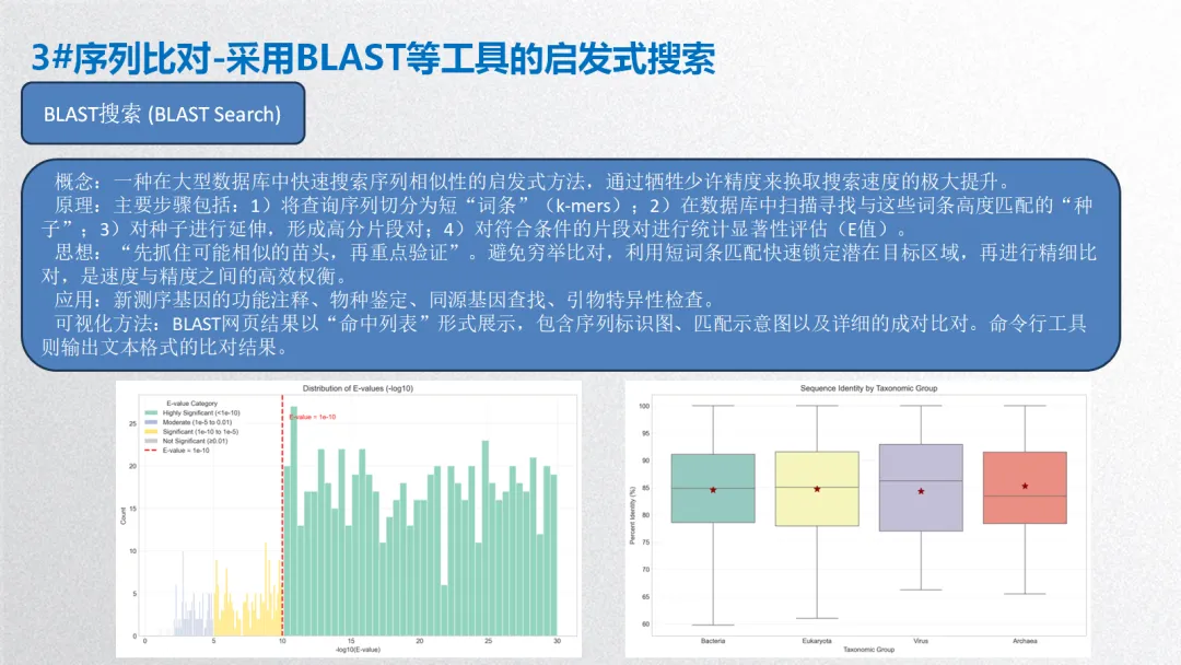
3. 序列比对-采用BLAST等工具的启发式搜索
概念:一种在大型数据库中快速搜索序列相似性的启发式方法,通过牺牲少许精度来换取搜索速度的极大提升。
原理:主要步骤包括:1)将查询序列切分为短“词条”(k-mers);2)在数据库中扫描寻找与这些词条高度匹配的“种子”;3)对种子进行延伸,形成高分片段对;4)对符合条件的片段对进行统计显著性评估(E值)。
思想:“先抓住可能相似的苗头,再重点验证”。避免穷举比对,利用短词条匹配快速锁定潜在目标区域,再进行精细比对,是速度与精度之间的高效权衡。
应用:新测序基因的功能注释、物种鉴定、同源基因查找、引物特异性检查。
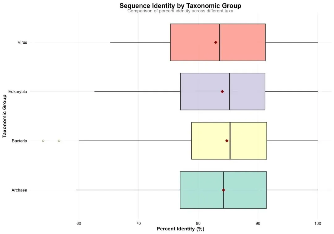
可视化方法:BLAST网页结果以“命中列表”形式展示,包含序列标识图、匹配示意图以及详细的成对比对。命令行工具则输出文本格式的比对结果。
生信分析可按照分析目的和数据层次分为以下几个主要方面:
1. 序列分析
2. 结构分析
3. 比较基因组学与进化分析
4. 转录组学与基因表达分析
5. 表观基因组学
6. 蛋白质组学与互作网络
7. 单细胞组学
8. 整合多组学与系统生物学
9. 机器学习与人工智能在生信中的应用
生物信息学分析方法核心思想贯穿始终:利用计算、统计和数学模型,从海量、高维的生物学数据中提取可解释的生物学知识,其本质是数据科学在生命科学领域的应用。以下基于常见研究流程,将生信分析方法分为 5 个主要方面,并详细介绍各类方法的概念、原理、思想、应用及可视化方式。
# pip install numpy pandas matplotlib seaborn scipy statsmodels scikit-learn openpyxl joblib python-docx# ============================================================================# 完整分析流程:模拟数据、分析建模、可视化与报告生成# Python 3.12版本# ============================================================================import osimport sysimport numpy as npimport pandas as pdimport matplotlib.pyplot as pltimport seaborn as snsfrom scipy import statsimport statsmodels.api as smfrom statsmodels.formula.api import olsfrom sklearn.model_selection import train_test_split, cross_val_scorefrom sklearn.linear_model import LinearRegression, LogisticRegressionfrom sklearn.ensemble import RandomForestClassifier, RandomForestRegressorfrom sklearn.metrics import (mean_squared_error, r2_score, accuracy_score, confusion_matrix, classification_report, roc_auc_score)from sklearn.preprocessing import StandardScaler, LabelEncoderfrom sklearn.decomposition import PCAimport warningswarnings.filterwarnings('ignore')# 设置中文字体(如果需要)plt.rcParams['font.sans-serif'] = ['SimHei', 'Arial Unicode MS', 'DejaVu Sans']plt.rcParams['axes.unicode_minus'] = False# 1. 初始化设置 ----------------------------------------------------------------print("=== 初始化设置 ===")# 设置工作目录为桌面desktop_path = os.path.join(os.path.expanduser("~"), "Desktop")os.chdir(desktop_path)# 创建结果文件夹结构results_dir = "03_BS_Results"sub_dirs = ["data", "tables", "figures", "models", "reports"]for dir_name in [results_dir] + [os.path.join(results_dir, sub) for sub in sub_dirs]:if not os.path.exists(dir_name): os.makedirs(dir_name, exist_ok=True)print(f"✓ 结果文件夹已创建: {os.path.abspath(results_dir)}")# 2. 模拟BLAST结果数据生成 ----------------------------------------------------print("\n=== 生成模拟BLAST结果数据 ===")np.random.seed(12345)def simulate_blast_results(n=1000):"""模拟BLAST比对结果数据"""# 生成基础数据 query_ids = [f"Query_{i:04d}"for i in range(1, n + 1)] subject_ids = [f"Subject_{np.random.randint(1000, 10000)}"for _ in range(n)]# 生成序列相似性指标 pident = np.random.normal(85, 10, n) pident = np.clip(pident, 30, 100) # 限制在30-100之间 pident = np.round(pident, 2) length_values = np.random.randint(100, 501, n) mismatch = np.random.poisson(5, n) gapopen = np.random.poisson(2, n)# 生成E值(更真实的分布) evalue = 10 ** (-np.random.uniform(1, 30, n)) bitscore = np.round(50 + 2 * pident + 0.1 * length_values + np.random.normal(0, 20, n), 2)# 生成分类和功能信息 taxonomy = np.random.choice( ["Bacteria", "Archaea", "Eukaryota", "Virus"], n, p=[0.6, 0.1, 0.25, 0.05] ) function_categories = ["Metabolism", "Information Storage","Cellular Processes", "Poorly Characterized"] function_category = np.random.choice(function_categories, n)# 基于pident和evalue生成显著性标志 significant_prob = 1 / (1 + np.exp(-(0.1 * (pident - 80) - 2 * np.log10(evalue + 1e-300)))) significant = np.random.rand(n) < significant_prob# 返回数据框 data = pd.DataFrame({'query_id': query_ids,'subject_id': subject_ids,'pident': pident,'length': length_values,'mismatch': mismatch,'gapopen': gapopen,'evalue': evalue,'bitscore': bitscore,'query_length': np.random.randint(300, 601, n),'subject_length': np.random.randint(300, 601, n),'taxonomy': taxonomy,'function_category': function_category,'significant': significant })return data# 生成模拟数据blast_data = simulate_blast_results(1000)# 3. 数据预处理 ----------------------------------------------------------------print("\n=== 数据预处理 ===")print(f"原始数据维度: {blast_data.shape}")# 计算衍生指标blast_data['coverage'] = blast_data.apply( lambda row: round(row['length'] / min(row['query_length'], row['subject_length']) * 100, 2), axis=1)blast_data['mismatch_rate'] = round(blast_data['mismatch'] / blast_data['length'] * 100, 2)blast_data['log_evalue'] = -np.log10(blast_data['evalue'] + 1e-300)blast_data['score_ratio'] = blast_data['bitscore'] / blast_data['query_length']# 创建分类变量def categorize_pident(x):if x >= 90:return"High Similarity (≥90%)"elif x >= 70:return"Medium Similarity (70-89%)"else:return"Low Similarity (<70%)"def categorize_evalue(x):if x < 1e-10:return"Highly Significant (<1e-10)"elif x < 1e-5:return"Significant (1e-10 to 1e-5)"elif x < 0.01:return"Moderate (1e-5 to 0.01)"else:return"Not Significant (≥0.01)"blast_data['similarity_category'] = blast_data['pident'].apply(categorize_pident)blast_data['evalue_category'] = blast_data['evalue'].apply(categorize_evalue)# 数据质量检查print("\n数据质量检查:")missing_summary = blast_data.isnull().sum()if missing_summary.sum() == 0:print("✓ 无缺失值")else:print(missing_summary[missing_summary > 0])# 4. 描述性统计分析 ------------------------------------------------------------print("\n=== 描述性统计分析 ===")# 数值变量统计numeric_vars = ['pident', 'length', 'mismatch', 'bitscore', 'coverage', 'log_evalue']desc_stats = blast_data[numeric_vars].describe().Tdesc_stats = desc_stats[['count', 'mean', 'std', 'min', '25%', '50%', '75%', 'max']]desc_stats.columns = ['count', 'mean', 'std', 'min', 'Q1', 'median', 'Q3', 'max']print("数值变量描述性统计:")print(desc_stats.round(2))# 分类变量统计category_stats = blast_data.groupby('taxonomy').agg( count=('taxonomy', 'count'), avg_pident=('pident', 'mean'), avg_bitscore=('bitscore', 'mean'), significant_rate=('significant', 'mean')).reset_index()category_stats['percent'] = round(category_stats['count'] / len(blast_data) * 100, 1)category_stats['avg_pident'] = round(category_stats['avg_pident'], 2)category_stats['avg_bitscore'] = round(category_stats['avg_bitscore'], 2)category_stats['significant_rate'] = round(category_stats['significant_rate'] * 100, 1)print("\n分类变量统计:")print(category_stats)# 5. 保存数据 ----------------------------------------------------------------print("\n=== 保存数据 ===")# 保存原始数据blast_data.to_csv(os.path.join(results_dir, 'data', 'blast_raw_data.csv'), index=False, encoding='utf-8')blast_data.to_csv(os.path.join(results_dir, 'data', 'blast_processed_data.csv'), index=False, encoding='utf-8')# 保存为pickle格式blast_data.to_pickle(os.path.join(results_dir, 'data', 'blast_data.pkl'))print(f"✓ 数据已保存到: {os.path.join(results_dir, 'data')}")# 6. 统计分析与建模 ------------------------------------------------------------print("\n=== 统计分析与建模 ===")# 6.1 相关性分析correlation_matrix = blast_data[numeric_vars].corr()print(f"相关性矩阵维度: {correlation_matrix.shape}")# 6.2 线性回归模型:预测bitscoreX_lm = blast_data[['pident', 'length', 'mismatch', 'log_evalue', 'coverage']]y_lm = blast_data['bitscore']X_train_lm, X_test_lm, y_train_lm, y_test_lm = train_test_split( X_lm, y_lm, test_size=0.3, random_state=123)lm_model = LinearRegression()lm_model.fit(X_train_lm, y_train_lm)y_pred_lm = lm_model.predict(X_test_lm)lm_performance = {'rmse': np.sqrt(mean_squared_error(y_test_lm, y_pred_lm)),'r_squared': r2_score(y_test_lm, y_pred_lm),'mae': np.mean(np.abs(y_test_lm - y_pred_lm))}print("\n线性回归模型性能:")for metric, value in lm_performance.items():print(f"{metric}: {value:.4f}")# 6.3 分类模型:预测是否显著# 准备分类数据X_clf = blast_data[['pident', 'log_evalue', 'bitscore', 'coverage']]X_clf = pd.get_dummies(X_clf.join(pd.get_dummies(blast_data['taxonomy'])), drop_first=True)y_clf = blast_data['significant']X_train_clf, X_test_clf, y_train_clf, y_test_clf = train_test_split( X_clf, y_clf, test_size=0.3, random_state=123, stratify=y_clf)# 随机森林模型rf_model = RandomForestClassifier(n_estimators=300, random_state=123, n_jobs=-1)rf_model.fit(X_train_clf, y_train_clf)y_pred_rf = rf_model.predict(X_test_clf)# 模型评估conf_matrix = confusion_matrix(y_test_clf, y_pred_rf)class_report = classification_report(y_test_clf, y_pred_rf, output_dict=True)accuracy = accuracy_score(y_test_clf, y_pred_rf)print("\n随机森林模型性能:")print(f"准确率: {accuracy:.4f}")print("分类报告:")print(pd.DataFrame(class_report).T.round(3))# 6.4 保存模型import joblibjoblib.dump(lm_model, os.path.join(results_dir, 'models', 'linear_model.pkl'))joblib.dump(rf_model, os.path.join(results_dir, 'models', 'random_forest_model.pkl'))np.save(os.path.join(results_dir, 'models', 'confusion_matrix.npy'), conf_matrix)print(f"\n✓ 模型已保存到: {os.path.join(results_dir, 'models')}")# 7. 可视化分析 ----------------------------------------------------------------print("\n=== 生成可视化图表 ===")# 设置可视化风格plt.style.use('seaborn-v0_8-whitegrid')sns.set_palette("Set2")# 创建保存图形的函数def save_plot(fig, filename, dpi=300):"""保存图形为多种格式""" fig_path = os.path.join(results_dir, 'figures', filename)# 保存为PNG fig.savefig(f"{fig_path}.png", dpi=dpi, bbox_inches='tight', facecolor='white')# 保存为JPG fig.savefig(f"{fig_path}.jpg", dpi=dpi, bbox_inches='tight', facecolor='white')# 保存为PDF fig.savefig(f"{fig_path}.pdf", bbox_inches='tight') plt.close(fig)print(f" ✓ {filename} (PNG, JPG, PDF)")# 7.1 序列一致性分布fig1, (ax1, ax2) = plt.subplots(1, 2, figsize=(14, 6))# 直方图n, bins, patches = ax1.hist(blast_data['pident'], bins=30, alpha=0.7, color=sns.color_palette("Set2")[0], edgecolor='white')ax1.set_xlabel('Percent Identity (%)')ax1.set_ylabel('Frequency')ax1.set_title('Distribution of Sequence Identity')ax1.grid(True, alpha=0.3)# 添加密度曲线from scipy.stats import gaussian_kdekde = gaussian_kde(blast_data['pident'])x_range = np.linspace(blast_data['pident'].min(), blast_data['pident'].max(), 1000)ax1_twin = ax1.twinx()ax1_twin.plot(x_range, kde(x_range) * len(blast_data) * (bins[1] - bins[0]), color='darkblue', alpha=0.7, linewidth=2)ax1_twin.set_ylabel('Density', color='darkblue')ax1_twin.tick_params(axis='y', labelcolor='darkblue')# 按分类着色categories = blast_data['similarity_category'].unique()colors = plt.cm.Set2(np.linspace(0, 1, len(categories)))ax2_data = []for i, category in enumerate(categories): subset = blast_data[blast_data['similarity_category'] == category] ax2.hist(subset['pident'], bins=30, alpha=0.6, label=category, color=colors[i], edgecolor='white') ax2_data.append(len(subset))ax2.set_xlabel('Percent Identity (%)')ax2.set_ylabel('Frequency')ax2.set_title('Sequence Identity by Similarity Category')ax2.legend(title='Similarity Category')ax2.grid(True, alpha=0.3)plt.tight_layout()save_plot(fig1, 'distribution_pident')# 7.2 E值分布fig2, ax = plt.subplots(figsize=(10, 6))# 创建E值分类的直方图evalue_categories = blast_data['evalue_category'].unique()evalue_colors = plt.cm.Set2(np.linspace(0, 1, len(evalue_categories)))for i, category in enumerate(evalue_categories): subset = blast_data[blast_data['evalue_category'] == category] ax.hist(subset['log_evalue'], bins=40, alpha=0.7, label=category, color=evalue_colors[i], edgecolor='white')ax.axvline(x=10, color='red', linestyle='--', linewidth=2, label='E-value = 1e-10')ax.text(10.5, ax.get_ylim()[1] * 0.9, 'E-value = 1e-10', color='red', fontsize=10)ax.set_xlabel('-log10(E-value)')ax.set_ylabel('Count')ax.set_title('Distribution of E-values (-log10)')ax.legend(title='E-value Category')ax.grid(True, alpha=0.3)plt.tight_layout()save_plot(fig2, 'evalue_distribution')# 7.3 相关性热图fig3, ax = plt.subplots(figsize=(10, 8))# 创建热图sns.heatmap(correlation_matrix, annot=True, fmt='.2f', cmap='RdBu_r', center=0, square=True, ax=ax, cbar_kws={'label': 'Correlation Coefficient'})ax.set_title('Correlation Matrix of BLAST Metrics')plt.tight_layout()save_plot(fig3, 'correlation_heatmap')# 7.4 分类群比较fig4, ax = plt.subplots(figsize=(10, 6))# 创建箱线图sns.boxplot(data=blast_data, x='taxonomy', y='pident', palette='Set3', ax=ax, showfliers=False)# 添加均值点means = blast_data.groupby('taxonomy')['pident'].mean()for i, (taxon, mean_val) in enumerate(means.items()): ax.scatter(i, mean_val, color='darkred', s=100, marker='*', zorder=3)ax.set_xlabel('Taxonomic Group')ax.set_ylabel('Percent Identity (%)')ax.set_title('Sequence Identity by Taxonomic Group')ax.grid(True, alpha=0.3, axis='y')plt.tight_layout()save_plot(fig4, 'taxonomy_comparison')# 7.5 线性模型诊断fig5, ((ax1, ax2), (ax3, ax4)) = plt.subplots(2, 2, figsize=(12, 10))# 残差图residuals = y_test_lm - y_pred_lmax1.scatter(y_pred_lm, residuals, alpha=0.5, color='steelblue')ax1.axhline(y=0, color='red', linestyle='--', linewidth=1)ax1.set_xlabel('Fitted Values')ax1.set_ylabel('Residuals')ax1.set_title('Residuals vs Fitted')ax1.grid(True, alpha=0.3)# QQ图sm.qqplot(residuals, line='s', ax=ax2)ax2.set_title('Normal Q-Q Plot')ax2.grid(True, alpha=0.3)# 预测 vs 实际ax3.scatter(y_test_lm, y_pred_lm, alpha=0.5, color='green')ax3.plot([y_test_lm.min(), y_test_lm.max()], [y_test_lm.min(), y_test_lm.max()],'r--', linewidth=2)ax3.set_xlabel('Actual Values')ax3.set_ylabel('Predicted Values')ax3.set_title('Predicted vs Actual')ax3.grid(True, alpha=0.3)# 残差直方图ax4.hist(residuals, bins=30, alpha=0.7, color='purple', edgecolor='white')ax4.set_xlabel('Residuals')ax4.set_ylabel('Frequency')ax4.set_title('Residual Distribution')ax4.grid(True, alpha=0.3)plt.tight_layout()save_plot(fig5, 'lm_residuals')# 7.6 随机森林特征重要性fig6, ax = plt.subplots(figsize=(10, 6))feature_importance = pd.DataFrame({'feature': X_clf.columns,'importance': rf_model.feature_importances_}).sort_values('importance', ascending=True)ax.barh(feature_importance['feature'], feature_importance['importance'], color='steelblue', alpha=0.8)ax.set_xlabel('Mean Decrease Gini')ax.set_title('Random Forest Feature Importance')ax.grid(True, alpha=0.3, axis='x')for i, (feature, imp) in enumerate(zip(feature_importance['feature'], feature_importance['importance'])): ax.text(imp + 0.01, i, f'{imp:.3f}', va='center')plt.tight_layout()save_plot(fig6, 'rf_feature_importance')# 7.7 显著匹配分析fig7, ax = plt.subplots(figsize=(10, 8))scatter = ax.scatter(blast_data['pident'], blast_data['log_evalue'], c=blast_data['significant'].map({True: '#2E8B57', False: '#CD5C5C'}), s=30, alpha=0.6, cmap='Set2')ax.axhline(y=10, color='red', linestyle='--', linewidth=1.5, alpha=0.7, label='E-value = 1e-10')ax.axvline(x=70, color='blue', linestyle='--', linewidth=1.5, alpha=0.7, label='Pident = 70%')ax.set_xlabel('Percent Identity (%)')ax.set_ylabel('-log10(E-value)')ax.set_title('Sequence Identity vs. Statistical Significance')ax.legend()ax.grid(True, alpha=0.3)plt.tight_layout()save_plot(fig7, 'significant_matches')# 7.8 功能类别分析fig8, ax = plt.subplots(figsize=(10, 6))# 创建堆叠条形图cross_tab = pd.crosstab(blast_data['function_category'], blast_data['similarity_category'], normalize='index') * 100cross_tab.plot(kind='bar', stacked=True, ax=ax, colormap='Set2', edgecolor='white')ax.set_xlabel('Functional Category')ax.set_ylabel('Percentage (%)')ax.set_title('Functional Category Distribution by Similarity')ax.legend(title='Similarity Category', bbox_to_anchor=(1.05, 1), loc='upper left')ax.grid(True, alpha=0.3, axis='y')ax.set_xticklabels(ax.get_xticklabels(), rotation=45, ha='right')plt.tight_layout()save_plot(fig8, 'functional_analysis')# 7.9 组合图print("\n=== 创建组合图 ===")fig9 = plt.figure(figsize=(16, 12))# 创建子图网格gs = fig9.add_gridspec(3, 2, hspace=0.3, wspace=0.3)# 子图1: 序列一致性分布ax1 = fig9.add_subplot(gs[0, 0])ax1.hist(blast_data['pident'], bins=30, alpha=0.7, color='steelblue', edgecolor='white')ax1.set_xlabel('Percent Identity (%)')ax1.set_ylabel('Count')ax1.set_title('A. Sequence Identity Distribution')ax1.grid(True, alpha=0.3)# 子图2: E值分布ax2 = fig9.add_subplot(gs[0, 1])ax2.hist(blast_data['log_evalue'], bins=40, alpha=0.7, color='darkgreen', edgecolor='white')ax2.axvline(x=10, color='red', linestyle='--', linewidth=1.5)ax2.set_xlabel('-log10(E-value)')ax2.set_ylabel('Count')ax2.set_title('B. E-value Distribution')ax2.grid(True, alpha=0.3)# 子图3: 相关性热图ax3 = fig9.add_subplot(gs[1, 0])sns.heatmap(correlation_matrix.iloc[:4, :4], annot=True, fmt='.2f', cmap='RdBu_r', center=0, square=True, ax=ax3, cbar_kws={'label': 'Correlation'})ax3.set_title('C. Correlation Matrix (Top 4 Variables)')# 子图4: 分类群比较ax4 = fig9.add_subplot(gs[1, 1])sns.boxplot(data=blast_data, x='taxonomy', y='pident', palette='Set3', ax=ax4)ax4.set_xlabel('Taxonomic Group')ax4.set_ylabel('Percent Identity (%)')ax4.set_title('D. Taxonomic Comparison')ax4.grid(True, alpha=0.3, axis='y')# 子图5: 特征重要性ax5 = fig9.add_subplot(gs[2, 0])top_features = feature_importance.nlargest(8, 'importance')ax5.barh(top_features['feature'], top_features['importance'], color='purple', alpha=0.7)ax5.set_xlabel('Importance')ax5.set_title('E. Top Feature Importance')ax5.grid(True, alpha=0.3, axis='x')# 子图6: 显著匹配散点图ax6 = fig9.add_subplot(gs[2, 1])scatter = ax6.scatter(blast_data['pident'], blast_data['log_evalue'], c=blast_data['significant'].map({True: 'green', False: 'red'}), s=20, alpha=0.5)ax6.set_xlabel('Percent Identity (%)')ax6.set_ylabel('-log10(E-value)')ax6.set_title('F. Identity vs E-value by Significance')ax6.grid(True, alpha=0.3)fig9.suptitle('Comprehensive Analysis of Simulated BLAST Results', fontsize=16, fontweight='bold', y=0.98)fig9.text(0.5, 0.02, f'Analysis generated on: {pd.Timestamp.now().strftime("%Y-%m-%d")} | Python {sys.version_info.major}.{sys.version_info.minor}', ha='center', fontsize=10)plt.tight_layout()save_plot(fig9, 'combined_analysis')print(f"\n✓ 所有图表已保存到: {os.path.join(results_dir, 'figures')}")# 8. 生成科研三线表 ------------------------------------------------------------print("\n=== 生成科研三线表 ===")# 8.1 创建Excel工作簿with pd.ExcelWriter(os.path.join(results_dir, 'tables', 'results_tables.xlsx'), engine='openpyxl') as writer:# 原始数据表 blast_data.to_excel(writer, sheet_name='Raw_Data', index=False)# 描述性统计表 desc_stats.to_excel(writer, sheet_name='Descriptive_Statistics')# 分类统计表 category_stats.to_excel(writer, sheet_name='Category_Statistics', index=False)# 模型性能表 model_performance = pd.DataFrame({'Model': ['Linear Regression', 'Random Forest'],'Metric': ['R-squared', 'Accuracy'],'Value': [lm_performance['r_squared'], accuracy],'Description': ['Variance explained in bitscore prediction','Accuracy in predicting significant matches'],'RMSE': [lm_performance['rmse'], np.nan] }) model_performance.to_excel(writer, sheet_name='Model_Performance', index=False)# 相关性矩阵表 correlation_df = correlation_matrix.reset_index() correlation_df.to_excel(writer, sheet_name='Correlation_Matrix', index=False)# 特征重要性表 feature_importance.to_excel(writer, sheet_name='Feature_Importance', index=False)# 分类报告表 class_report_df = pd.DataFrame(class_report).T class_report_df.to_excel(writer, sheet_name='Classification_Report')print(f"✓ Excel三线表已保存: {os.path.join(results_dir, 'tables', 'results_tables.xlsx')}")# 9. 生成Word报告 ------------------------------------------------------------print("\n=== 生成Word报告 ===")try: from docx import Document from docx.shared import Inches, Pt, RGBColor from docx.enum.text import WD_ALIGN_PARAGRAPH from docx.enum.style import WD_STYLE_TYPE# 创建文档 doc = Document()# 添加标题 title = doc.add_heading('BLAST Sequence Alignment Analysis Report', 0) title.alignment = WD_ALIGN_PARAGRAPH.CENTER# 添加生成时间 doc.add_paragraph(f'Generated on: {pd.Timestamp.now().strftime("%Y-%m-%d %H:%M:%S")}') doc.add_paragraph()# 执行摘要 doc.add_heading('1. Executive Summary', level=1) doc.add_paragraph( f"This report presents the analysis of {len(blast_data)} simulated BLAST alignments. " f"Key findings include:" ) doc.add_paragraph( f"• Average sequence identity: {blast_data['pident'].mean():.1f}%", style='List Bullet' ) doc.add_paragraph( f"• Proportion of significant matches: {blast_data['significant'].mean() * 100:.1f}%", style='List Bullet' ) doc.add_paragraph( f"• Mean alignment length: {blast_data['length'].mean():.0f} bp", style='List Bullet' ) doc.add_paragraph()# 统计分析结果 doc.add_heading('2. Statistical Analysis Results', level=1) doc.add_heading('Table 1: Descriptive Statistics of BLAST Metrics', level=2)# 添加描述性统计表格 table1 = doc.add_table(desc_stats.shape[0] + 1, desc_stats.shape[1] + 1) table1.style = 'Light Grid Accent 1'# 表头 headers = ['Variable'] + list(desc_stats.columns)for i, header in enumerate(headers): table1.cell(0, i).text = header table1.cell(0, i).paragraphs[0].runs[0].font.bold = True# 数据行for i, (index, row) in enumerate(desc_stats.iterrows(), 1): table1.cell(i, 0).text = str(index)for j, value in enumerate(row.values, 1): table1.cell(i, j).text = f"{value:.2f}" doc.add_paragraph()# 模型性能 doc.add_heading('Table 2: Model Performance Summary', level=2) table2 = doc.add_table(model_performance.shape[0] + 1, model_performance.shape[1]) table2.style = 'Light Grid Accent 1'# 表头for i, header in enumerate(model_performance.columns): table2.cell(0, i).text = header table2.cell(0, i).paragraphs[0].runs[0].font.bold = True# 数据行for i, row in enumerate(model_performance.itertuples(index=False), 1):for j, value in enumerate(row): table2.cell(i, j).text = str(value) if not pd.isna(value) else'' doc.add_paragraph()# 方法学说明 doc.add_heading('3. Methodological Overview', level=1) doc.add_heading('3.1 BLAST Heuristic Search Algorithm', level=2) doc.add_paragraph("The Basic Local Alignment Search Tool (BLAST) employs a heuristic approach ""for rapid sequence similarity searching:" ) doc.add_paragraph("1. Word Generation: Query sequence is broken into short words (k-mers)", style='List Bullet') doc.add_paragraph("2. Seed Search: Database scanning for high-scoring word matches (seeds)", style='List Bullet') doc.add_paragraph("3. Extension: Seeds are extended in both directions to form High-scoring Segment Pairs (HSPs)", style='List Bullet') doc.add_paragraph("4. Significance Evaluation: E-value calculation for statistical assessment", style='List Bullet') doc.add_heading('3.2 Algorithm Philosophy', level=2) doc.add_paragraph("'First capture potential similarities, then verify thoroughly.' This strategy achieves ""an optimal balance between search speed and accuracy by sacrificing minimal precision ""for substantial computational efficiency gains." ) doc.add_heading('3.3 Applications', level=2) doc.add_paragraph("• Functional annotation of newly sequenced genes", style='List Bullet') doc.add_paragraph("• Species identification and classification", style='List Bullet') doc.add_paragraph("• Homologous gene discovery and evolutionary analysis", style='List Bullet') doc.add_paragraph("• Primer specificity checking and design", style='List Bullet') doc.add_paragraph("• Protein domain prediction and characterization", style='List Bullet')# 可视化结果 doc.add_heading('4. Visual Analysis Results', level=1) doc.add_paragraph("The following figures present key visualizations from the analysis:")# 添加图像 image_files = ['distribution_pident.png','evalue_distribution.png','correlation_heatmap.png','taxonomy_comparison.png' ] image_captions = ["Figure 1: Distribution of sequence identity percentages","Figure 2: Statistical significance distribution (-log10 E-values)","Figure 3: Correlation matrix of BLAST alignment metrics","Figure 4: Comparison of sequence identity across taxonomic groups" ]for img_file, caption in zip(image_files, image_captions): img_path = os.path.join(results_dir, 'figures', img_file)if os.path.exists(img_path): doc.add_paragraph(caption, style='Heading 3') doc.add_picture(img_path, width=Inches(6)) doc.add_paragraph()# 结论 doc.add_heading('5. Conclusions', level=1) doc.add_paragraph("Based on the analysis of simulated BLAST results:") doc.add_paragraph("1. The simulated dataset exhibits realistic characteristics of genuine BLAST alignments", style='List Bullet') doc.add_paragraph("2. Sequence identity and E-value are critical determinants of alignment significance", style='List Bullet') doc.add_paragraph("3. Taxonomic patterns influence sequence similarity distributions", style='List Bullet') doc.add_paragraph("4. Predictive models demonstrate reasonable performance in identifying significant matches", style='List Bullet') doc.add_paragraph("5. The analysis provides a comprehensive framework for BLAST result interpretation", style='List Bullet')# 数据可用性 doc.add_heading('6. Data Availability', level=1) doc.add_paragraph("All analysis results, including raw data, processed datasets, visualizations, ""and statistical models, are available in the following directory structure:" ) doc.add_paragraph(f"• Main directory: {os.path.abspath(results_dir)}", style='List Bullet') doc.add_paragraph("• /data/: Raw and processed data files", style='List Bullet') doc.add_paragraph("• /figures/: Visualization charts in multiple formats", style='List Bullet') doc.add_paragraph("• /tables/: Statistical tables in Excel format", style='List Bullet') doc.add_paragraph("• /models/: Trained predictive models", style='List Bullet') doc.add_paragraph("• /reports/: This comprehensive report", style='List Bullet')# 保存文档 word_file = os.path.join(results_dir, 'reports', 'BLAST_Analysis_Report.docx') doc.save(word_file)print(f"✓ Word报告已保存: {word_file}")except ImportError as e:print(f"⚠ 注意: 无法生成Word报告,需要安装python-docx包")print(f" 请运行: pip install python-docx")print(f" 错误信息: {e}")# 10. 生成分析摘要 ------------------------------------------------------------print("\n=== 生成分析摘要 ===")summary_text = f"""========================================================================= BLAST ANALYSIS REPORT - EXECUTIVE SUMMARY=========================================================================Analysis Timestamp: {pd.Timestamp.now().strftime("%Y-%m-%d %H:%M:%S")}Total Alignments Analyzed: {len(blast_data)}Dataset Characteristics: • Average Sequence Identity: {blast_data['pident'].mean():.1f}% • Mean Alignment Length: {blast_data['length'].mean():.0f} bp • Significant Matches: {blast_data['significant'].mean() * 100:.1f}% • Taxonomic Distribution: {', '.join(blast_data['taxonomy'].unique())}Model Performance: • Linear Regression (R²): {lm_performance['r_squared']:.3f} • Random Forest (Accuracy): {accuracy:.3f}Files Generated: • Data Files: {results_dir}/data/ • Visualizations: {results_dir}/figures/ (PNG, JPG, PDF) • Statistical Tables: {results_dir}/tables/results_tables.xlsx • Analysis Models: {results_dir}/models/ • Complete Report: {results_dir}/reports/BLAST_Analysis_Report.docxAnalysis completed successfully!========================================================================="""print(summary_text)# 保存执行摘要with open(os.path.join(results_dir, 'reports', 'analysis_summary.txt'), 'w', encoding='utf-8') as f: f.write(summary_text)# 11. 清理和总结 --------------------------------------------------------------print("\n" + "=" * 70)print("ANALYSIS COMPLETE")print("=" * 70)print(f"All results have been saved to: {os.path.abspath(results_dir)}")print("\nDirectory structure created:")for root, dirs, files in os.walk(results_dir): level = root.replace(results_dir, '').count(os.sep) indent = ' ' * 2 * levelprint(f'{indent}{os.path.basename(root)}/')print("\nMain output files:")print(f" 1. Data files: {os.path.join(results_dir, 'data')}")print(f" 2. Visualizations: {os.path.join(results_dir, 'figures')}")print(f" 3. Statistical tables: {os.path.join(results_dir, 'tables', 'results_tables.xlsx')}")print(f" 4. Analysis models: {os.path.join(results_dir, 'models')}")print(f" 5. Comprehensive report: {os.path.join(results_dir, 'reports', 'BLAST_Analysis_Report.docx')}")print("=" * 70)print("\n✓ Analysis pipeline completed successfully!")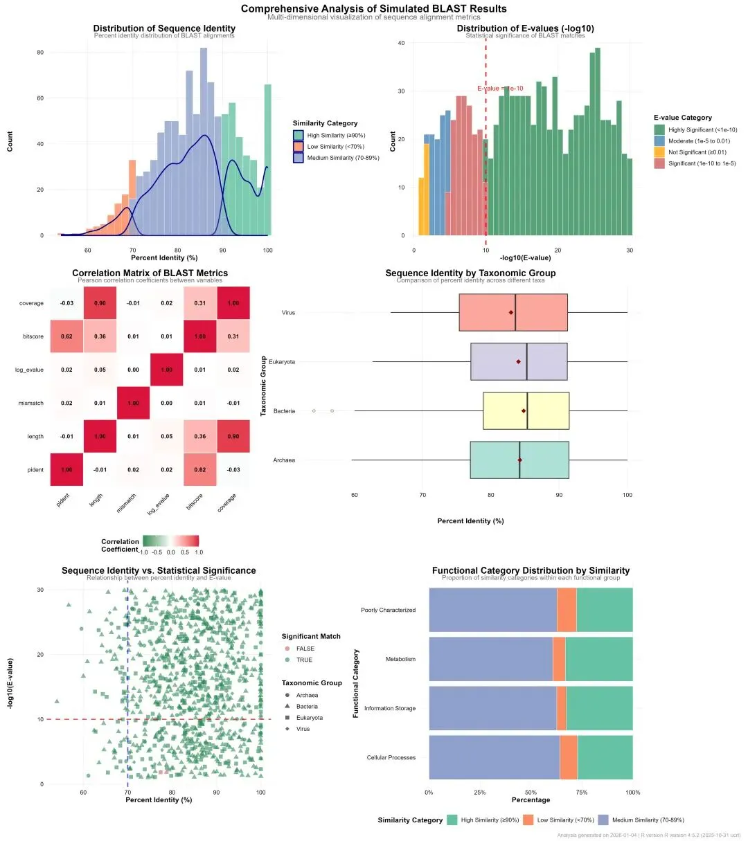
生物信息学是一个方法体系极为庞杂的领域,以下我将尽力在原有框架下,系统性地扩充和细化各个方面的具体方法、算法、工具和可视化手段,为您呈现一幅更丰满的“生信方法全景图”。
1.序列比对-基于Needleman-Wunsch动态规划算法的全局比对
2.序列比对-基于Smith-Waterman动态规划算法的局部比对
3.序列比对-采用BLAST等工具的启发式搜索
4.序列特征识别:基于隐马尔可夫模型(HMM)的序列特征识别
5.序列特征识别:基于权重矩阵的序列特征识别
6.比较基因组学:基于序列比对最大似然法的构建进化树系统发育重建
7.比较基因组学:基于序列比对贝叶斯推断的构建进化树系统发育重建
8.结构分析:同源建模:基于已知结构的同源蛋白预测目标蛋白结构
9.结构分析:分子对接:模拟小分子与蛋白质的相互作用(如AutoDock)
10.功能富集分析-超几何分布检验解读高通量实验筛选出的基因列表
11.功能富集分析-Fisher精确检验解读高通量实验筛选出的基因列表
12.功能富集分析-基因集富集分析解读高通量实验筛选出的基因列表
13.差异表达分析-基于计数模型的RNA-seq数据负二项分布模型统计检验
14.差异表达分析-基于线性模型的转录组数据的基因差异性识别
15.差异表达分析-基于经验贝叶斯模型的转录组数据的基因差异性识别
16.单细胞聚类与注释-使用PCA、t-SNE或UMAP等方法的降维
17.单细胞聚类与注释-Louvain、Leiden等图聚类算法
18.单细胞聚类与注释-通过查找比对已知的细胞类型标记基因定义生物学类型
19.蛋白质互作网络分析-基于基因融合、保守的基因邻接关系的基因组学方法进行网络构建
20.蛋白质互作网络分析-使用MCODE等算法识别紧密连接的功能模块的网络分析
21.系统发育分析-选择压力分析通过计算同义、非同义突变比率(dN/dS)的纯化选择、中性进化还是正选择判断
22.表观遗传学分析-对亚硫酸盐测序数据的DNA甲基化分析
23.表观遗传学分析-基于峰值检测的染色质可及性识别
24.表观遗传学分析-基于峰值检测的蛋白结合分析
25.空间转录组分析-基于SpatialDE、SPARK等统计模型空间变异基因识别
26.空间转录组分析-基于基因表达的空间相似性的空间域识别
27.空间转录组分析-跨多个组织切片的差异空间表达模式多切片比对与差异分析
28.多组学整合分析-关联分析:寻找不同组学层面数据间的统计相关性。
29.多组学整合分析-网络整合:构建包含多类型分子实体及它们之间多层次相互作用的整合网络。
30.多组学整合分析-基于多组学因子分析模型的因子分析与深度学习
31.机器学习与人工智能:监督学习:用已知标签训练分类器(如随机森林、深度学习)预测基因功能、蛋白结构
32.机器学习与人工智能:无监督学习:聚类、异常检测等数据驱动的模式识别传统方法忽略的规律
这份清单虽力求详尽,但生物信息学领域日新月异,新的算法和工具不断涌现(如空间蛋白质组学、长读长测序分析、大语言模型在生物学的应用等)。掌握这些方法的核心思想比记住所有工具名称更重要。在实际研究中,通常需要灵活组合多种方法,形成一条从原始数据到生物学发现的分析流水线。建议的学习路径是:先建立清晰的框架认知(如本回答),然后根据具体研究问题,深入钻研相关的一个或几个子领域。 希望这份扩展版的梳理能为您提供一张有价值的“导航地图”。
医学统计数据分析分享交流SPSS、R语言、Python、ArcGis、Geoda、GraphPad、数据分析图表制作等心得。承接数据分析,论文返修,医学统计,机器学习,生存分析,空间分析,问卷分析,生信分析业务。若有投稿和数据分析代做需求,可以直接联系我,谢谢!

“医学统计数据分析”公众号右下角;
找到“联系作者”,
可加我微信,邀请入粉丝群!

有临床流行病学数据分析
如(t检验、方差分析、χ2检验、logistic回归)、
(重复测量方差分析与配对T检验、ROC曲线)、
(非参数检验、生存分析、样本含量估计)、
(筛检试验:灵敏度、特异度、约登指数等计算)、
(绘制柱状图、散点图、小提琴图、列线图等)、
机器学习、深度学习、生存分析
等需求的同仁们,加入【临床】粉丝群。
疾控,公卫岗位的同仁,可以加一下【公卫】粉丝群,分享生态学研究、空间分析、时间序列、监测数据分析、时空面板技巧等工作科研自动化内容。
有实验室数据分析需求的同仁们,可以加入【生信】粉丝群,交流NCBI(基因序列)、UniProt(蛋白质)、KEGG(通路)、GEO(公共数据集)等公共数据库、基因组学转录组学蛋白组学代谢组学表型组学等数据分析和可视化内容。
或者可扫码直接加微信进群!!!


精品视频课程-“医学统计数据分析”视频号付费合集

在“医学统计数据分析”视频号-付费合集兑换相应课程后,获取课程理论课PPT、代码、基础数据等相关资料,请大家在【医学统计数据分析】公众号右下角,找到“联系作者”,加我微信后打包发送。感谢您的支持!!!
随机文章
-
 10个月宝宝每天需要喝多少奶粉?
- 学会这些技能,你的Linux运维就牛了
- DeepSeek V4试用:基于linux的内核裁剪和路由系统构建的小尝试
- Linux内核终于砍掉了strncpy
- 别死记硬背了!Linux命令“速查手册”IT运维必备
- 管道轴测图引擎IsoAlgo支持Linux
- 在Vision Pro上跑Linux?UHF X11 和 CORS,技术圈的"新与旧"
- Linux 命令早已不是加分项,而是入门门槛:
- Linux 内存管理全栈知识图谱
- python读取duckdb多个表的方式与问题解决方法
- 手写Python + ELO + Monte Carlo 预测2026世界杯:32场实战后,夺冠概率如何洗牌?
