双锥面型砂轮轮廓的几何建模与Python可视化

在精密磨削加工中，砂轮轮廓的精确描述对磨削质量与容屑性能具有决定性影响。双锥面型砂轮因其特有的两侧锥角与圆弧过渡结构，能够有效平衡磨削效率与砂轮寿命，广泛应用于成形磨削和切入磨削。为深入理解该轮廓的几何构成，本文基于表1所示的轮廓表达式，利用Python编程实现完整轮廓曲线的生成与可视化，并对每一段几何元素进行数学推导与代码实现剖析。

一、轮廓的几何参数与坐标计算

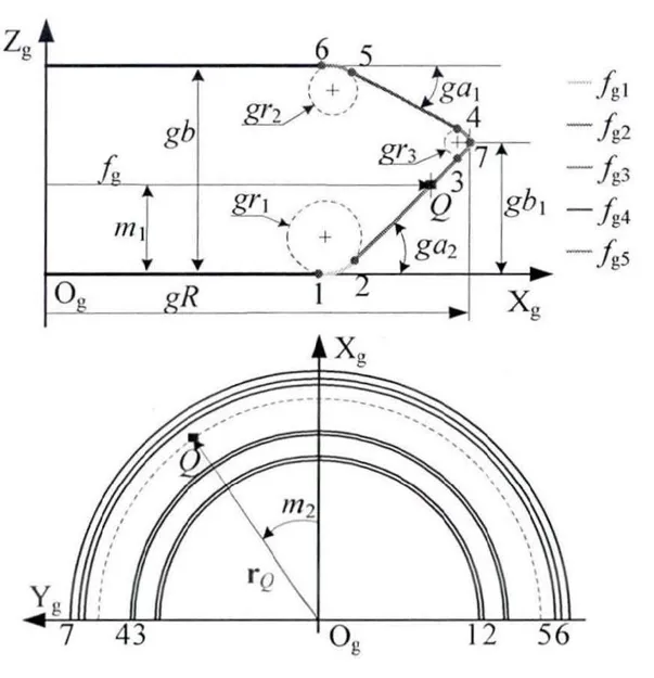
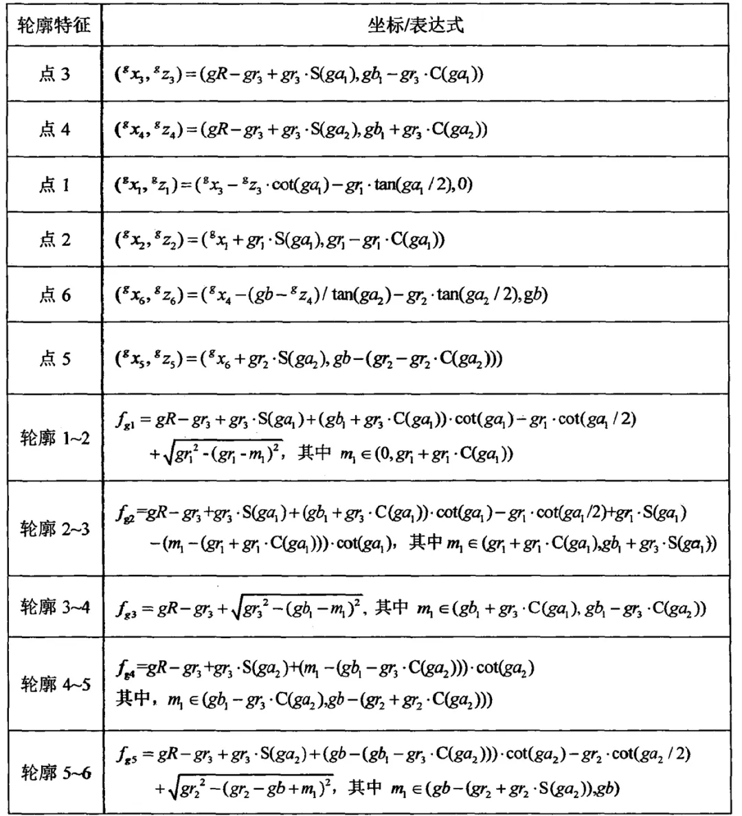
表1所定义的轮廓由六个关键点（点1至点6）和五段轮廓线（圆弧1‑2、直线2‑3、圆弧3‑4、直线4‑5、圆弧5‑6）组成。轮廓所在的坐标系为砂轮轴向截面坐标系，其中轴代表径向（砂轮半径方向），轴代表轴向（砂轮宽度方向）。所有几何关系均基于以下给定参数：

• • 砂轮基圆半径 （单位：mm）；
• • 左侧锥角 （表中记为），右侧锥角 （）；
• • 左侧过渡圆弧半径 （），右侧过渡圆弧半径 （），中间圆弧半径 （）；
• • 砂轮总宽度 ，中间圆弧圆心轴向偏移 。

表1中的公式采用大量三角函数和几何约束，其核心思想是：先由圆弧3‑4（圆心，半径）确定点3和点4的位置；再由点3沿锥角方向通过直线和圆弧1‑2反推点1、点2；由点4沿锥角方向通过直线和圆弧5‑6反推点5、点6。这样，整个轮廓就被六个点完整定义，且各段之间满足切向连续（圆弧与直线相切）。

具体坐标计算如下（角度全部转换为弧度）：

• • 点3：；
• • 点4：；
• • 点1：由点3向左侧锥面直线投影，并考虑圆弧1‑2的切点关系，其坐标为，坐标为0；
• • 点2：由圆弧1‑2（圆心，半径）上角度为的切点，；
• • 点6：对称地，由点4向右侧锥面投影，并考虑圆弧5‑6的切点关系，，；
• • 点5：圆弧5‑6（圆心，半径）上的切点，。

所有角度均以砂轮轴线为基准，正方向为逆时针。

二、分段轮廓的数学表示

表1中给出了五段轮廓的表达式，它们均以参数（沿轴向的变量）表示径向坐标。这些表达式实际上描述了每段上与的映射关系，但更直接的可视化方法是使用参数方程：对圆弧采用圆心角参数，对直线采用线性插值。本文采用后者，因为它更直观且易于编程。

圆弧1‑2

圆心，半径。点1对应角度，点2对应角度。因此圆弧上任意点可写为：

直线2‑3

直接对和进行线性插值，两端点为点2和点3。

圆弧3‑4

圆心，半径。点3和点4的角度通过反正切函数求得，然后在此区间内均匀采样。

直线4‑5

线性插值连接点4和点5。

圆弧5‑6

圆心，半径。点5和点6的角度同样由坐标反算，并在此区间采样。

采用上述参数化方式，可以生成任意密度的轮廓点集，从而获得高精度的图形。

三、Python完整实现（主绘图程序）

以下代码完全依据上述几何关系，独立计算所有关键点坐标并绘制完整的砂轮轴向截面轮廓。该代码块可直接运行，仅依赖numpy和matplotlib两个基础科学计算库。

import numpy as np
import matplotlib.pyplot as plt

# ====================== 参数赋值 ======================
gR = 50.0
ga1_deg = 10.0
ga2_deg = 20.0
gr1 = 10.0
gr2 = 15.0
gr3 = 3.0
gb = 15.0
gb1 = 7.0

# 角度转弧度
ga1 = np.radians(ga1_deg)
ga2 = np.radians(ga2_deg)

sin1, cos1 = np.sin(ga1), np.cos(ga1)
tan1 = np.tan(ga1)
cot1 = 1.0 / tan1
tan_half1 = np.tan(ga1 / 2.0)

sin2, cos2 = np.sin(ga2), np.cos(ga2)
tan2 = np.tan(ga2)
cot2 = 1.0 / tan2
tan_half2 = np.tan(ga2 / 2.0)

# ====================== 关键点坐标 ======================
# 点3
gx3 = gR - gr3 + gr3 * sin1
gz3 = gb1 - gr3 * cos1

# 点4
gx4 = gR - gr3 + gr3 * sin2
gz4 = gb1 + gr3 * cos2

# 点1
gx1 = gx3 - gz3 * cot1 - gr1 * tan_half1
gz1 = 0.0

# 点2
gx2 = gx1 + gr1 * sin1
gz2 = gr1 - gr1 * cos1

# 点6
gx6 = gx4 - (gb - gz4) * cot2 - gr2 * tan_half2
gz6 = gb

# 点5
gx5 = gx6 + gr2 * sin2
gz5 = gb - (gr2 - gr2 * cos2)

# ====================== 分段生成轮廓点 ======================
n_arc = 80# 圆弧采样点数
n_line = 30# 直线采样点数

# 1. 圆弧 1~2
O1x, O1z = gx1, gr1
theta1_start = -np.pi / 2.0
theta1_end = ga1 - np.pi / 2.0
theta1 = np.linspace(theta1_start, theta1_end, n_arc)
arc1_x = O1x + gr1 * np.cos(theta1)
arc1_z = O1z + gr1 * np.sin(theta1)

# 2. 直线 2~3
line23_x = np.linspace(gx2, gx3, n_line)
line23_z = np.linspace(gz2, gz3, n_line)

# 3. 圆弧 3~4
O3x, O3z = gR - gr3, gb1
theta3_start = np.arctan2(gz3 - O3z, gx3 - O3x)
theta3_end = np.arctan2(gz4 - O3z, gx4 - O3x)
theta3 = np.linspace(theta3_start, theta3_end, n_arc)
arc3_x = O3x + gr3 * np.cos(theta3)
arc3_z = O3z + gr3 * np.sin(theta3)

# 4. 直线 4~5
line45_x = np.linspace(gx4, gx5, n_line)
line45_z = np.linspace(gz4, gz5, n_line)

# 5. 圆弧 5~6
O5x, O5z = gx6, 0.0
theta5_start = np.arctan2(gz5 - O5z, gx5 - O5x)
theta5_end = np.arctan2(gz6 - O5z, gx6 - O5x)
theta5 = np.linspace(theta5_start, theta5_end, n_arc)
arc5_x = O5x + gr2 * np.cos(theta5)
arc5_z = O5z + gr2 * np.sin(theta5)

# 合并所有点
x_all = np.concatenate([arc1_x, line23_x, arc3_x, line45_x, arc5_x])
z_all = np.concatenate([arc1_z, line23_z, arc3_z, line45_z, arc5_z])

# ====================== 绘图 ======================
plt.figure(figsize=(10, 7))
plt.plot(x_all, z_all, 'b-', linewidth=2.5, label='砂轮轮廓')

# 标记关键点
points_x = [gx1, gx2, gx3, gx4, gx5, gx6]
points_z = [gz1, gz2, gz3, gz4, gz5, gz6]
plt.plot(points_x, points_z, 'ro', markersize=7, label='关键点')

# 标注点编号
labels = ['1', '2', '3', '4', '5', '6']
for i, (x, z) inenumerate(zip(points_x, points_z)):
    ha = 'right'if i < 3else'left'
    va = 'bottom'if i in [0, 5] else'top'
    plt.text(x, z, f'P{labels[i]}', fontsize=12, ha=ha, va=va)

plt.xlabel('径向坐标 $x$ (mm)', fontsize=13)
plt.ylabel('轴向坐标 $z$ (mm)', fontsize=13)
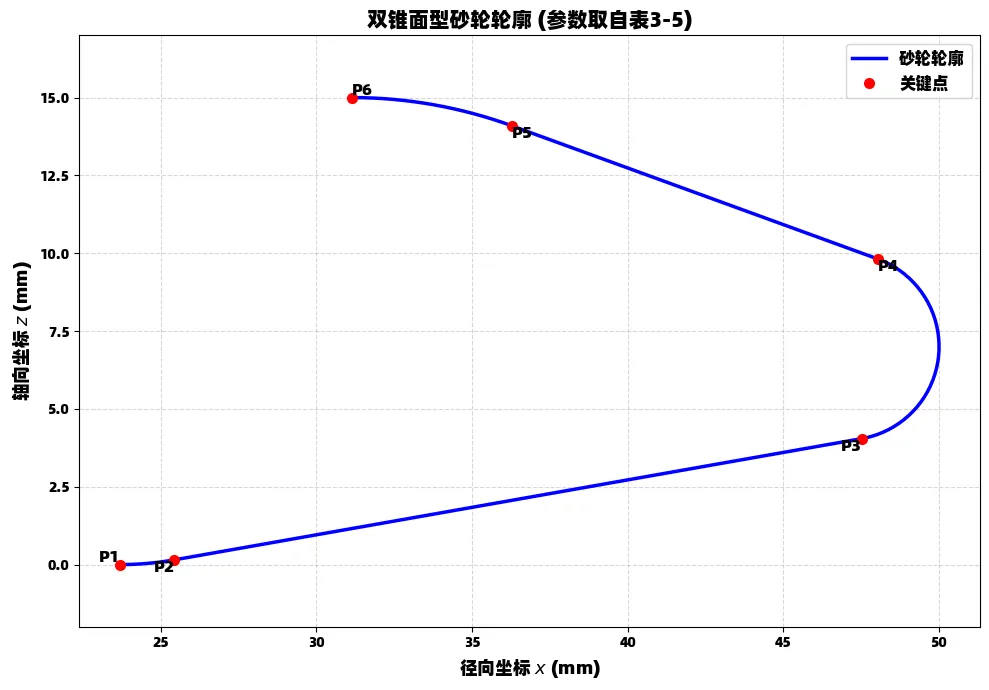
plt.title('双锥面型砂轮轮廓 (参数取自表3‑5)', fontsize=15)
plt.grid(True, linestyle='--', alpha=0.5)
plt.axis('equal')
plt.legend(fontsize=12)
plt.tight_layout()
plt.show()

运行上述代码，将得到一幅清晰的砂轮轮廓图，图中蓝色曲线为连续轮廓，红色圆点标记六个关键点，并标注了序号。由于采用等比例坐标轴，各圆弧和直线的几何关系得以真实呈现。

四、独立输出关键点坐标的辅助程序

为了便于数值校核，以下代码独立于绘图程序，仅计算六个关键点的坐标并以表格形式打印。该代码块不依赖绘图库，可单独运行，直接验证公式计算的正确性。

import numpy as np

# 参数（与主程序一致）
gR, ga1_deg, ga2_deg = 50.0, 10.0, 20.0
gr1, gr2, gr3 = 10.0, 15.0, 3.0
gb, gb1 = 15.0, 7.0

ga1, ga2 = np.radians(ga1_deg), np.radians(ga2_deg)
sin1, cos1 = np.sin(ga1), np.cos(ga1)
sin2, cos2 = np.sin(ga2), np.cos(ga2)
cot1, cot2 = 1.0 / np.tan(ga1), 1.0 / np.tan(ga2)
tan_half1, tan_half2 = np.tan(ga1/2), np.tan(ga2/2)

# 计算各点
gx3 = gR - gr3 + gr3 * sin1
gz3 = gb1 - gr3 * cos1
gx4 = gR - gr3 + gr3 * sin2
gz4 = gb1 + gr3 * cos2
gx1 = gx3 - gz3 * cot1 - gr1 * tan_half1
gz1 = 0.0
gx2 = gx1 + gr1 * sin1
gz2 = gr1 - gr1 * cos1
gx6 = gx4 - (gb - gz4) * cot2 - gr2 * tan_half2
gz6 = gb
gx5 = gx6 + gr2 * sin2
gz5 = gb - (gr2 - gr2 * cos2)

points = {
'点1': (gx1, gz1),
'点2': (gx2, gz2),
'点3': (gx3, gz3),
'点4': (gx4, gz4),
'点5': (gx5, gz5),
'点6': (gx6, gz6)
}

print("关键点坐标 (x, z):")
for name, (x, z) in points.items():
print(f"{name}: ({x:.4f}, {z:.4f})")

该程序输出结果可直接与表3‑3中的表达式对照，是验证建模正确性的有效工具。

五、轮廓几何特征分析

从生成的图形可见，砂轮轮廓在轴向（方向）从0到 mm范围内变化，径向（方向）最大半径接近基圆半径 mm。左侧锥角较小（10°），对应的圆弧1‑2半径较大（），使得左侧刃口过渡平缓；右侧锥角较大（20°），过渡圆弧半径也较大（），有利于排屑。中间圆弧3‑4半径很小（），但它在连接左右两侧锥面时提供了光滑过渡，避免了尖角应力集中。各段衔接点处（点2‑3、点4‑5）的切线斜率连续，保证了磨削过程中砂轮表面力学的均匀性。

通过调整参数（如、锥角、圆弧半径等），可以快速生成不同形状的砂轮廓形，为磨削工艺优化提供数值依据。本文提供的代码具有良好的可扩展性，读者可自行修改参数或增加轮廓评价模块，例如计算容屑槽面积、接触弧长等。

总之，基于表1的几何表达式，结合Python科学计算与可视化能力，我们建立了一套完整、自洽的双锥面砂轮轮廓建模与绘图工具。该方法不仅准确再现了理论轮廓，也为后续磨削运动学仿真和砂轮磨损分析奠定了图形基础。