从零开始的脑电分析:MNE-Python 指南
- 2026-07-07 06:35:46
从零开始的脑电分析:MNE-Python 指南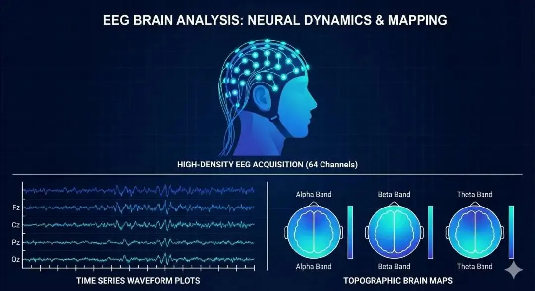


一篇搞定脑电数据预处理、ERP、时频分析与统计检验的全流程教程
📌 写在前面
脑电(EEG)技术因其高时间分辨率,成为认知神经科学研究的首选工具。但面对高密度电极、长时段记录的海量数据,如何进行单变量大规模分析(Mass Univariate Analysis)成为研究者的核心挑战。
所谓"单变量",指的是对每个电极-时间点(或电极-频率)独立进行统计检验;而"大规模"则意味着我们同时进行成千上万次检验——比如64个电极 × 500个时间点 = 32,000次检验!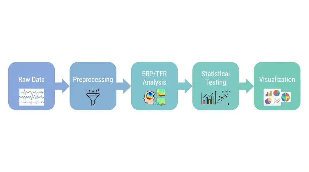 这带来的挑战是多重比较问题:如果设定 p < 0.05,单纯进行32,000次检验会期望产生1600个假阳性!因此,我们需要特殊的统计校正方法。
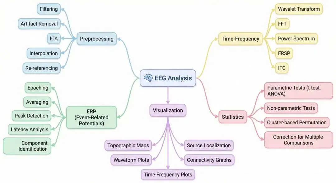
本教程将完整介绍基于 MNE-Python 的分析流程:
数据导入 → 预处理 → ERP分析 → 时频分析 → 统计检验 → 可视化
第一部分:环境准备
安装 MNE-Python
# 完整安装(推荐)
pip install mne[full]

# 或使用 conda
conda install -c conda-forge mne
核心依赖
import numpy as np
import matplotlib.pyplot as plt
import mne
from mne import Epochs
from mne.preprocessing import ICA
from mne.stats import permutation_cluster_test
from mne.time_frequency import tfr_morlet
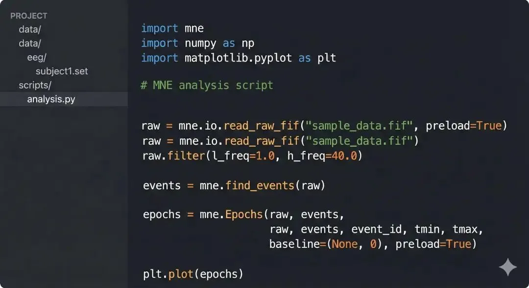
第二部分:数据导入
MNE 支持几乎所有主流脑电数据格式:
read_raw_brainvision() | ||
read_raw_eeglab() | ||
read_raw_cnt() | ||
read_raw_edf() |
快速读取
import mne

# 读取 BrainVision 格式(最常用)
raw = mne.io.read_raw_brainvision(
'subject_01.vhdr',
    preload=True# 预加载到内存
)

# 设置电极位置(10-20系统)
montage = mne.channels.make_standard_montage('standard_1020')
raw.set_montage(montage)
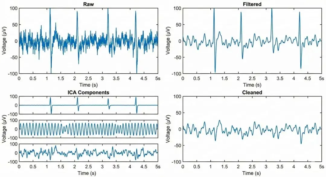
第三部分:预处理流程
预处理是脑电分析的基础,直接影响后续结果的质量。以下是标准流程:
┌─────────────┐    ┌─────────────┐    ┌─────────────┐
│   重参考    │ → │   滤波      │ → │   ICA去伪迹 │
└─────────────┘    └─────────────┘    └─────────────┘
       ↓                                      ↓
┌─────────────┐    ┌─────────────┐    ┌─────────────┐
│   分段      │ → │  基线校正   │ → │  拒绝坏段   │
└─────────────┘    └─────────────┘    └─────────────┘
3.1 重参考与滤波
# 平均参考(最常用)
raw.set_eeg_reference('average')

# 带通滤波 0.5-40 Hz
raw.filter(l_freq=0.5, h_freq=40.)

# 陷波滤波去除50Hz工频干扰
raw.notch_filter(freqs=50)
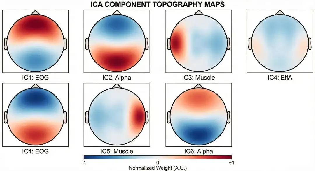
3.2 ICA 去除眼电伪迹
# 创建ICA对象
ica = ICA(n_components=20, method='picard', random_state=42)
ica.fit(raw)

# 自动检测眼电成分
eog_epochs = mne.preprocessing.create_eog_epochs(raw)
eog_indices, _ = ica.find_bads_eog(eog_epochs)
ica.exclude = eog_indices

# 应用ICA
raw_clean = ica.apply(raw.copy())
3.3 数据分段
# 定义事件
events = mne.find_events(raw)
event_id = {'experimental': 1, 'control': 2}

# 创建 Epochs
epochs = Epochs(
    raw_clean,
    events,
    event_id,
    tmin=-0.2,     # 刺激前200ms
    tmax=0.8,      # 刺激后800ms
    baseline=(-0.2, 0),  # 基线校正
    preload=True
)
第四部分:ERP分析
4.1 计算平均ERP
# 按条件平均
exp_evoked = epochs['experimental'].average()
ctrl_evoked = epochs['control'].average()

# 提取特定成分(如P3:250-500ms)
p3_window = (0.25, 0.5)
p3_channels = ['Pz', 'P3', 'P4']

# 计算均值振幅
p3_data = exp_evoked.copy().crop(*p3_window).data
p3_amp = p3_data.mean()
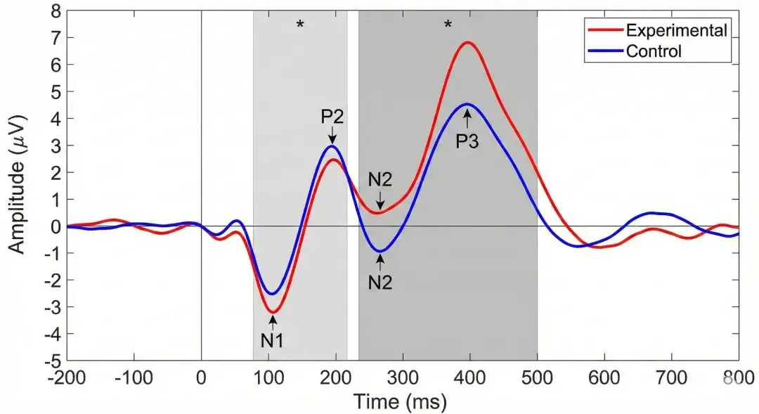
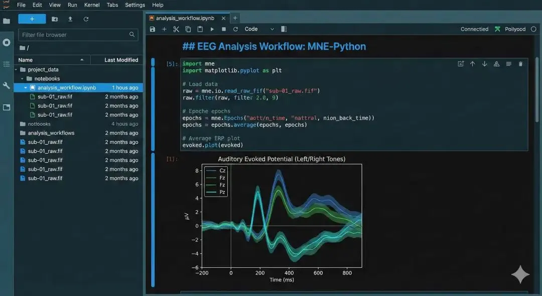
4.2 ERP可视化
# 波形对比
mne.viz.plot_compare_evokeds(
{'Experimental': exp_evoked, 'Control': ctrl_evoked},
picks=['Fz', 'Cz', 'Pz'],
colors={'Experimental': '#e74c3c', 'Control': '#3498db'}
)
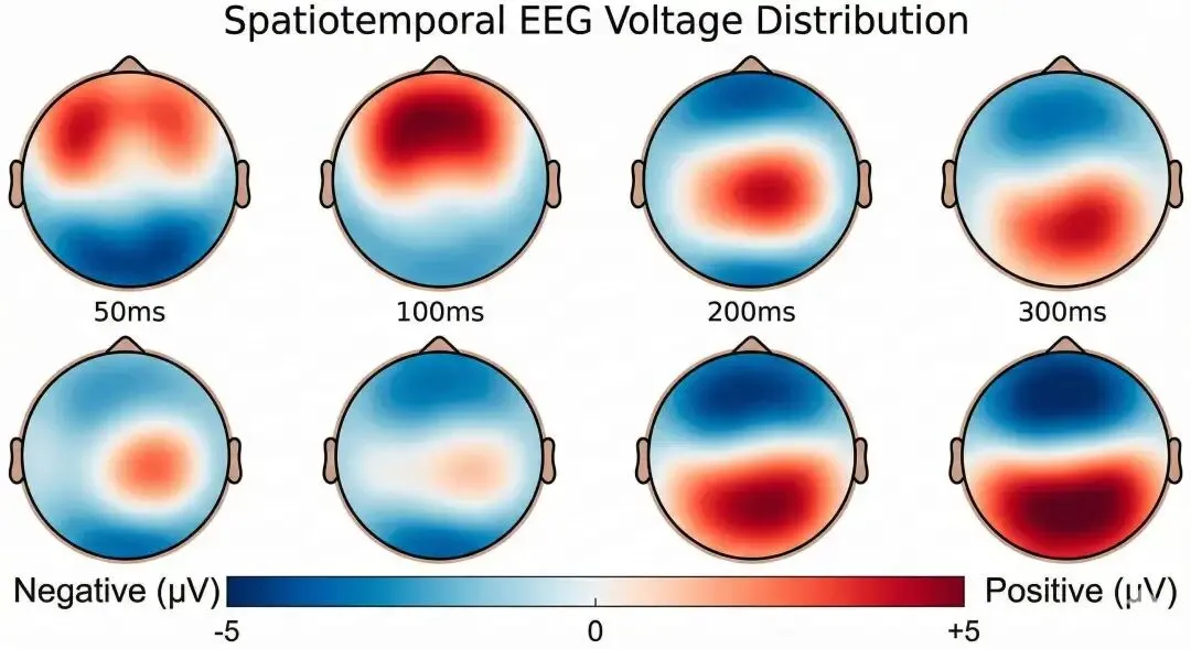
# 拓扑图(特定时间点)
times = [0.1, 0.2, 0.3, 0.4]
exp_evoked.plot_topomap(times=times)
ERP波形对比
ERP拓扑脑图序列
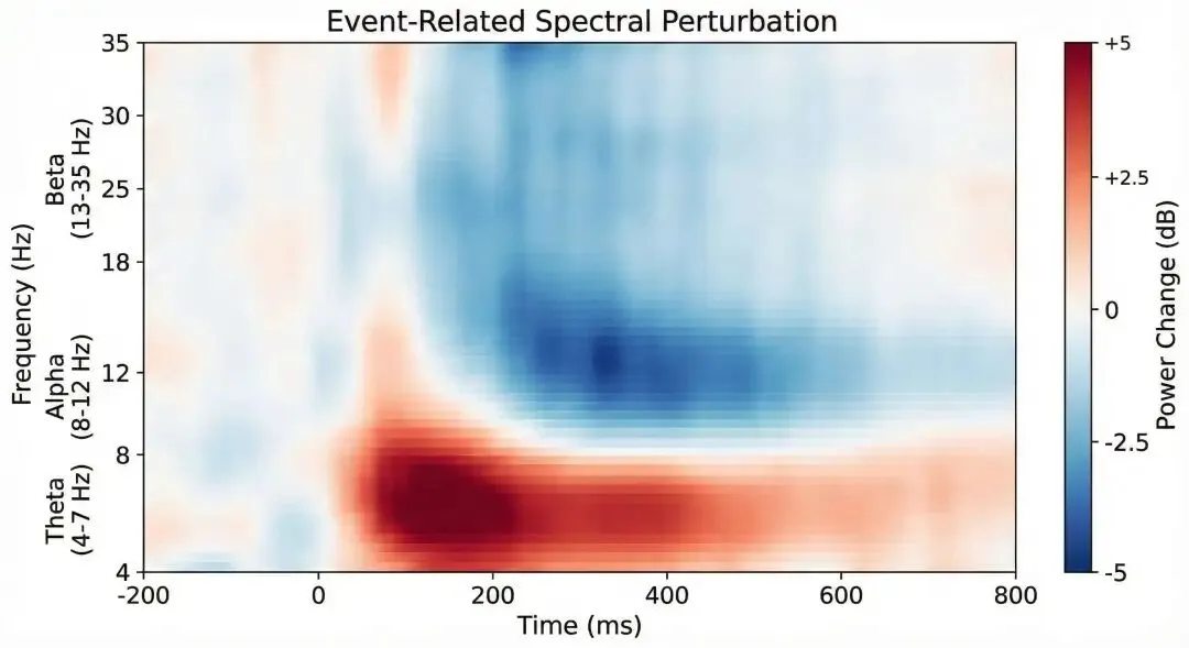
第五部分:时频分析
时频分析揭示EEG信号的频域特征随时间的变化。
5.1 计算时频功率
# Morlet小波变换
freqs = np.arange(4, 35, 2)  # 4-35 Hz
n_cycles = freqs / 2

power = tfr_morlet(
    epochs,
    freqs=freqs,
    n_cycles=n_cycles,
    average=True,
    return_itc=False
)

# 基线校正
power.apply_baseline(baseline=(-0.2, 0), mode='mean')
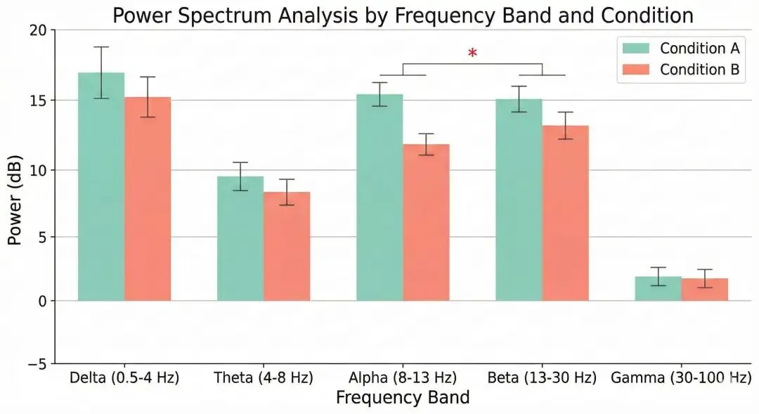
5.2 频带分析
# 定义经典频带
bands = {
'delta': (1, 4),
'theta': (4, 8),
'alpha': (8, 13),
'beta': (13, 30),
'gamma': (30, 50)
}
第六部分:统计检验
这是大规模分析的核心——如何正确处理多重比较问题。
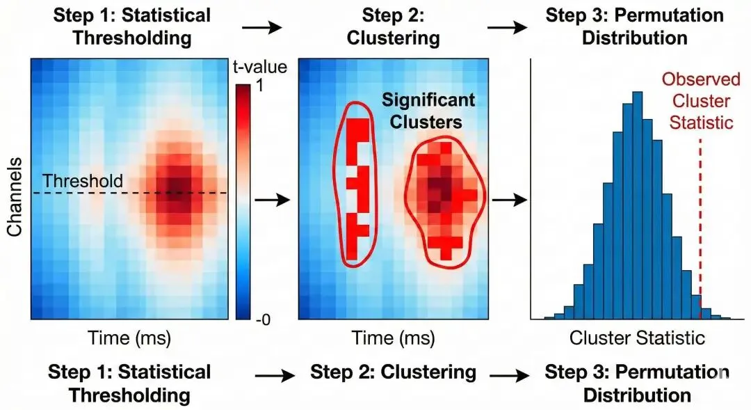
6.1 聚类排列检验 (Cluster-based Permutation Test)
这是EEG研究中使用最广泛的统计方法,由 Maris & Oostenveld (2007) 提出。
核心思想:
对每个电极-时间点计算 t 值 将相邻且超过阈值的点聚合成"聚类" 计算每个聚类的统计量(如 t 值之和) 通过排列检验获取 p 值
from mne.stats import permutation_cluster_test

# 准备数据
data_cond1 = epochs['experimental'].get_data()
data_cond2 = epochs['control'].get_data()

# 聚类排列检验
T_obs, clusters, p_values, H0 = permutation_cluster_test(
    [data_cond1, data_cond2],
    n_permutations=1000,  # 排列次数
    threshold=3.0,        # t阈值(约p<0.05)
    tail=0,               # 双尾检验
    n_jobs=-1# 并行计算
)

# 找显著聚类
significant_clusters = np.where(p_values < 0.05)[0]
print(f"发现 {len(significant_clusters)} 个显著聚类")
6.2 结果可视化
import matplotlib.pyplot as plt

# 绘制显著时间窗口
fig, ax = plt.subplots(figsize=(12, 4))
times = epochs.times

for cl_idx in significant_clusters:
    cluster = clusters[cl_idx]
    time_ind = cluster[1]
    ax.axvspan(
        times[time_ind[0]], times[time_ind[-1]],
        alpha=0.3, color='red',
        label=f'p={p_values[cl_idx]:.3f}'
    )

# 绘制t值曲线
ax.plot(times, T_obs[epochs.ch_names.index('Pz'), :])
ax.axhline(3.0, color='k', linestyle='--', label='阈值')
ax.set_xlabel('时间 (s)')
ax.set_ylabel('t 值')
ax.legend()
第七部分:完整代码示例
以下是一个可直接运行的完整脚本:
"""
脑电分析完整流程
=====================
作者: 脑电分析札记
日期: 2026
"""

import numpy as np
import matplotlib.pyplot as plt
import mne
from mne import Epochs, create_info
from mne.preprocessing import ICA
from mne.stats import permutation_cluster_test
from mne.time_frequency import tfr_morlet

# ──────────────────────────────────────
# 1. 数据加载
# ──────────────────────────────────────
raw = mne.io.read_raw_brainvision('data.vhdr', preload=True)

# 设置电极位置
montage = mne.channels.make_standard_montage('standard_1020')
raw.set_montage(montage)

# ──────────────────────────────────────
# 2. 预处理
# ──────────────────────────────────────
# 重参考
raw.set_eeg_reference('average')

# 滤波
raw.filter(0.5, 40., fir_design='firwin')
raw.notch_filter([50, 100])

# ICA去眼电
ica = ICA(n_components=20, method='picard', random_state=42)
ica.fit(raw)
eog_indices, _ = ica.find_bads_eog(raw)
ica.exclude = eog_indices
raw = ica.apply(raw)

# ──────────────────────────────────────
# 3. 分段
# ──────────────────────────────────────
events = mne.find_events(raw)
event_id = {'exp': 1, 'ctrl': 2}

epochs = Epochs(
    raw, events, event_id,
    tmin=-0.2, tmax=0.8,
    baseline=(-0.2, 0),
    preload=True,
    reject={'eeg': 150e-6}
)

# ──────────────────────────────────────
# 4. ERP分析
# ──────────────────────────────────────
exp_evoked = epochs['exp'].average()
ctrl_evoked = epochs['ctrl'].average()

# 可视化
mne.viz.plot_compare_evokeds(
    {'实验': exp_evoked, '对照': ctrl_evoked},
    picks=['Fz', 'Cz', 'Pz'],
    colors={'实验': '#e74c3c', '对照': '#3498db'}
)

# ──────────────────────────────────────
# 5. 时频分析
# ──────────────────────────────────────
power = tfr_morlet(
    epochs['exp'],
    freqs=np.arange(4, 35, 2),
    n_cycles=7,
    average=True
)
power.apply_baseline((-0.2, 0), mode='mean')

# 绘制时频图
power.plot(picks='Pz', baseline=(-0.2, 0))

# ──────────────────────────────────────
# 6. 统计检验
# ──────────────────────────────────────
data_exp = epochs['exp'].get_data()
data_ctrl = epochs['ctrl'].get_data()

T_obs, clusters, p_values, H0 = permutation_cluster_test(
    [data_exp, data_ctrl],
    n_permutations=1000,
    threshold=3.0,
    tail=0,
    n_jobs=-1
)

# 输出结果
for i, p in enumerate(p_values):
if p < 0.05:
        print(f"聚类 {i+1}: p = {p:.4f} **")

print("分析完成!")
进阶技巧
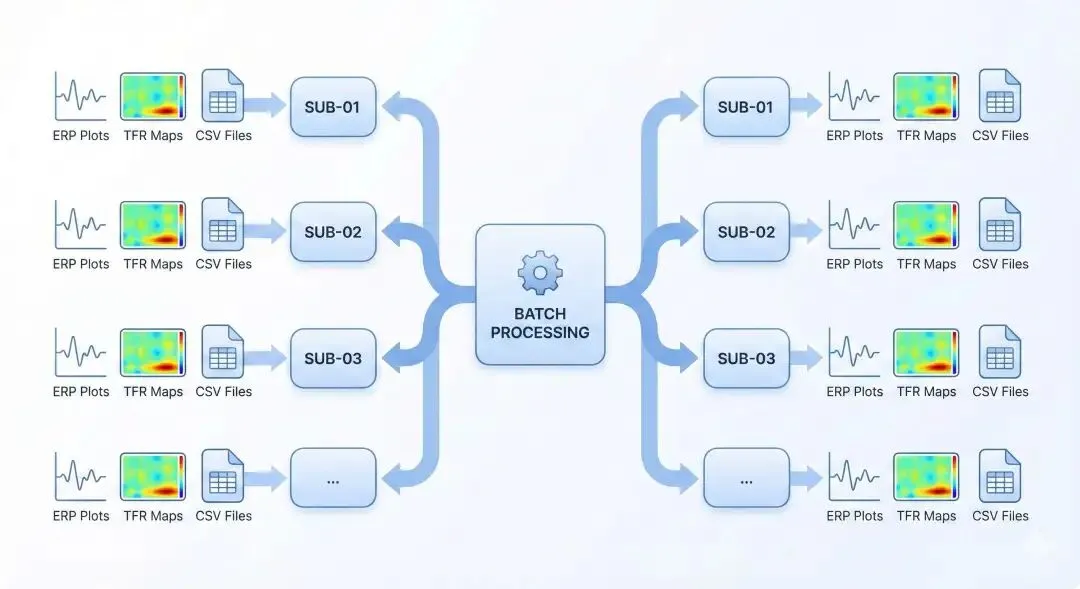
技巧1:批量处理多被试
import glob
from pathlib import Path

results = {}

for file in glob.glob('data/sub-*/eeg/*.vhdr'):
    sub_id = Path(file).parent.parent.name

# 加载和预处理
    raw = mne.io.read_raw_brainvision(file, preload=True)
# ... (预处理步骤)

# 分析并保存结果
    results[sub_id] = {
'p3_amplitude': p3_amp,
'n170_latency': n170_lat
    }
技巧2:自动检测坏通道
# 使用信噪比检测
noise_levels = raw.copy().filter(110, 140).get_data()
noise_levels = np.abs(noise_levels).mean(axis=1)

bad_channels = np.where(noise_levels > 2 * np.median(noise_levels))[0]
raw.info['bads'] = [raw.ch_names[i] for i in bad_channels]
raw.interpolate_bads()
总结
本教程介绍了基于 MNE-Python 的脑电单变量大规模分析完整流程:
| 预处理 | |
| ERP分析 | |
| 时频分析 | |
| 统计检验 |
进一步学习
MNE 官方文档: https://mne.tools/ Maris & Oostenveld (2007): 非参数统计检验经典论文 Cohen (2014): 《Analyzing Neural Time Series Data》
本文来自网友投稿或网络内容,如有侵犯您的权益请联系我们删除,联系邮箱:wyl860211@qq.com 。

