# pip install pandas numpy matplotlib seaborn statsmodels scipy scikit-learn joblib python-docximport osimport pandas as pdimport numpy as npimport matplotlib.pyplot as pltimport seaborn as snsfrom datetime import datetimeimport warningswarnings.filterwarnings('ignore')# 统计和模型相关库from statsmodels.tsa.stattools import adfuller, kpssfrom statsmodels.tsa.arima.model import ARIMAfrom statsmodels.graphics.tsaplots import plot_acf, plot_pacfimport scipy.stats as stats# 评估指标from sklearn.metrics import mean_squared_error, mean_absolute_error# 并行计算from joblib import Parallel, delayedimport multiprocessing# 报告生成from docx import Documentfrom docx.shared import Inchesclass TimeSeriesMAnalysis: def __init__(self):# 获取桌面路径并创建结果文件夹 self.desktop_path = os.path.join(os.path.expanduser("~"), "Desktop") self.results_path = os.path.join(self.desktop_path, "Results时间MA")# 创建子目录 self.subdirs = ["Models", "Plots", "Forecasts", "Diagnostics", "Word_Report","ACF_PACF_Plots", "Residual_Plots", "Model_Comparison" ]# 创建主目录和子目录if not os.path.exists(self.results_path): os.makedirs(self.results_path)for subdir in self.subdirs: subdir_path = os.path.join(self.results_path, subdir)if not os.path.exists(subdir_path): os.makedirs(subdir_path)# 设置matplotlib中文字体(尝试多种字体) plt.rcParams['font.sans-serif'] = ['SimHei', 'Microsoft YaHei', 'DejaVu Sans'] plt.rcParams['axes.unicode_minus'] = False# 初始化数据 self.combined_data = None self.train_data = None self.test_data = None self.model_results = None# 选择要分析的疾病 self.selected_diseases = ["influenza", "common_cold", "pneumonia","bacillary_dysentery", "hand_foot_mouth", "hemorrhagic_fever" ]print(f"结果将保存到: {self.results_path}") def load_data(self, file_path=None):"""加载数据"""if file_path is None:# 如果没有提供文件路径,创建示例数据 self._create_sample_data()else: try: self.combined_data = pd.read_csv(file_path)if'timestamp'in self.combined_data.columns: self.combined_data['timestamp'] = pd.to_datetime(self.combined_data['timestamp'])print(f"数据加载成功,共 {len(self.combined_data)} 行") except Exception as e:print(f"加载数据失败: {e},将使用示例数据") self._create_sample_data()# 划分训练集和测试集 self._split_data() def _create_sample_data(self):"""创建示例数据"""print("创建示例数据...") dates = pd.date_range('1981-01-01', '2025-12-31', freq='M') n = len(dates)# 创建模拟数据 np.random.seed(42) data = {'timestamp': dates }# 为每种疾病创建模拟时间序列for disease in self.selected_diseases:# 基础趋势 + 季节性 + 噪声 trend = np.linspace(0, 10, n) seasonal = 5 * np.sin(2 * np.pi * np.arange(n) / 12) noise = np.random.normal(0, 2, n)# 不同疾病有不同的模式if disease == "influenza": data[disease] = 50 + trend + 20 * seasonal + 10 * noiseelif disease == "common_cold": data[disease] = 100 + 0.5 * trend + 10 * seasonal + 15 * noiseelif disease == "pneumonia": data[disease] = 30 + 2 * trend + 8 * seasonal + 5 * noiseelif disease == "bacillary_dysentery": data[disease] = 20 + trend + 5 * seasonal + 3 * noiseelif disease == "hand_foot_mouth": data[disease] = 40 + 3 * trend + 12 * seasonal + 8 * noiseelse: # hemorrhagic_fever data[disease] = 10 + 0.2 * trend + 3 * seasonal + 2 * noise# 确保没有负值 data[disease] = np.maximum(data[disease], 0) self.combined_data = pd.DataFrame(data)print(f"示例数据创建完成,共 {len(self.combined_data)} 行") def _split_data(self):"""划分训练集和测试集"""# 确保数据已加载if self.combined_data is None: self._create_sample_data() train_start = '1981-01-01' train_end = '2015-12-31' test_start = '2016-01-01' test_end = '2025-12-31' self.train_data = self.combined_data[ (self.combined_data['timestamp'] >= train_start) & (self.combined_data['timestamp'] <= train_end) ].copy() self.test_data = self.combined_data[ (self.combined_data['timestamp'] >= test_start) & (self.combined_data['timestamp'] <= test_end) ].copy()print( f"训练集: {len(self.train_data)} 行, {self.train_data['timestamp'].min()} 至 {self.train_data['timestamp'].max()}")print( f"测试集: {len(self.test_data)} 行, {self.test_data['timestamp'].min()} 至 {self.test_data['timestamp'].max()}") def robust_stationarity_test(self, ts_data):"""稳健的平稳性检验"""# 处理常数序列if np.std(ts_data) == 0 or np.all(ts_data == ts_data[0]):return {'is_stationary': True,'adf_pvalue': 0.01,'kpss_pvalue': 0.1,'needs_diff': False }# 清理数据 clean_data = ts_data[~np.isnan(ts_data)]if len(clean_data) < 10:return {'is_stationary': False,'adf_pvalue': 1,'kpss_pvalue': 0,'needs_diff': True }# ADF检验 try: adf_result = adfuller(clean_data) adf_pvalue = adf_result[1] except: adf_pvalue = 1# KPSS检验 try: kpss_result = kpss(clean_data, regression='c') kpss_pvalue = kpss_result[1] except: kpss_pvalue = 0# 判断是否需要差分 needs_diff = (adf_pvalue > 0.05 or kpss_pvalue < 0.05)return {'is_stationary': not needs_diff,'adf_pvalue': adf_pvalue,'kpss_pvalue': kpss_pvalue,'needs_diff': needs_diff }

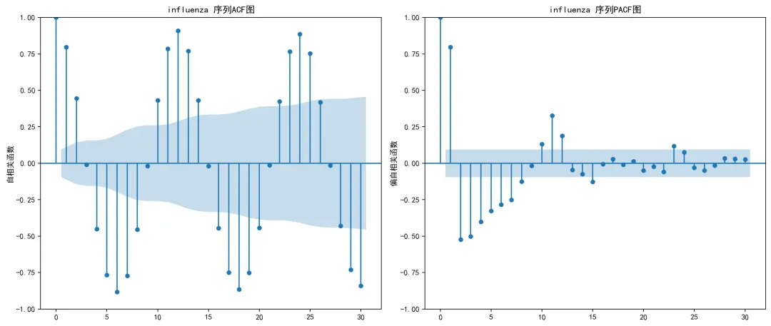
# 尝试其他阶数for q in range(2, max_q + 1): try: model = ARIMA(ts_data, order=(0, 0, q)).fit() current_aic = model.aicif current_aic < best_aic - 2: # AIC改进至少2个单位 best_aic = current_aic best_model = model best_q = q except Exception as e:continue# 忽略错误,继续尝试下一个qif best_model is None:# 如果所有尝试都失败,使用均值模型作为回退print("所有MA模型拟合失败,使用均值模型") mean_val = np.mean(ts_data)# 创建一个简单的类来模拟模型对象 class MeanModel: def __init__(self, mean_val, residuals): self.aic = np.nan self.bic = np.nan self.resid = residuals self.params = [mean_val] self.fittedvalues = np.full_like(residuals, mean_val) def forecast(self, steps):return np.full(steps, self.params[0]) def predict(self, start, end):return np.full(end - start, self.params[0]) best_model = MeanModel(mean_val, ts_data - mean_val) best_q = 0return {'model': best_model,'q': best_q,'aic': best_aic if hasattr(best_model, 'aic') else np.nan } def create_acf_pacf_plots(self, ts_data, disease, is_diff=False):"""生成ACF和PACF图""" try: fig, (ax1, ax2) = plt.subplots(1, 2, figsize=(14, 6))# ACF图 plot_acf(ts_data, ax=ax1, lags=30) title_suffix = "差分后"if is_diff else"" ax1.set_title(f'{disease} {title_suffix}序列ACF图') ax1.set_ylabel('自相关函数')# PACF图 plot_pacf(ts_data, ax=ax2, lags=30) ax2.set_title(f'{disease} {title_suffix}序列PACF图') ax2.set_ylabel('偏自相关函数') plt.tight_layout()# 保存图形 suffix = "_diff"if is_diff else"" plot_path = os.path.join(self.results_path, "ACF_PACF_Plots", f"ACF_PACF_{disease}{suffix}.png") plt.savefig(plot_path, dpi=200, bbox_inches='tight') plt.close()return fig except Exception as e:print(f"创建ACF/PACF图时出错: {e}")return None
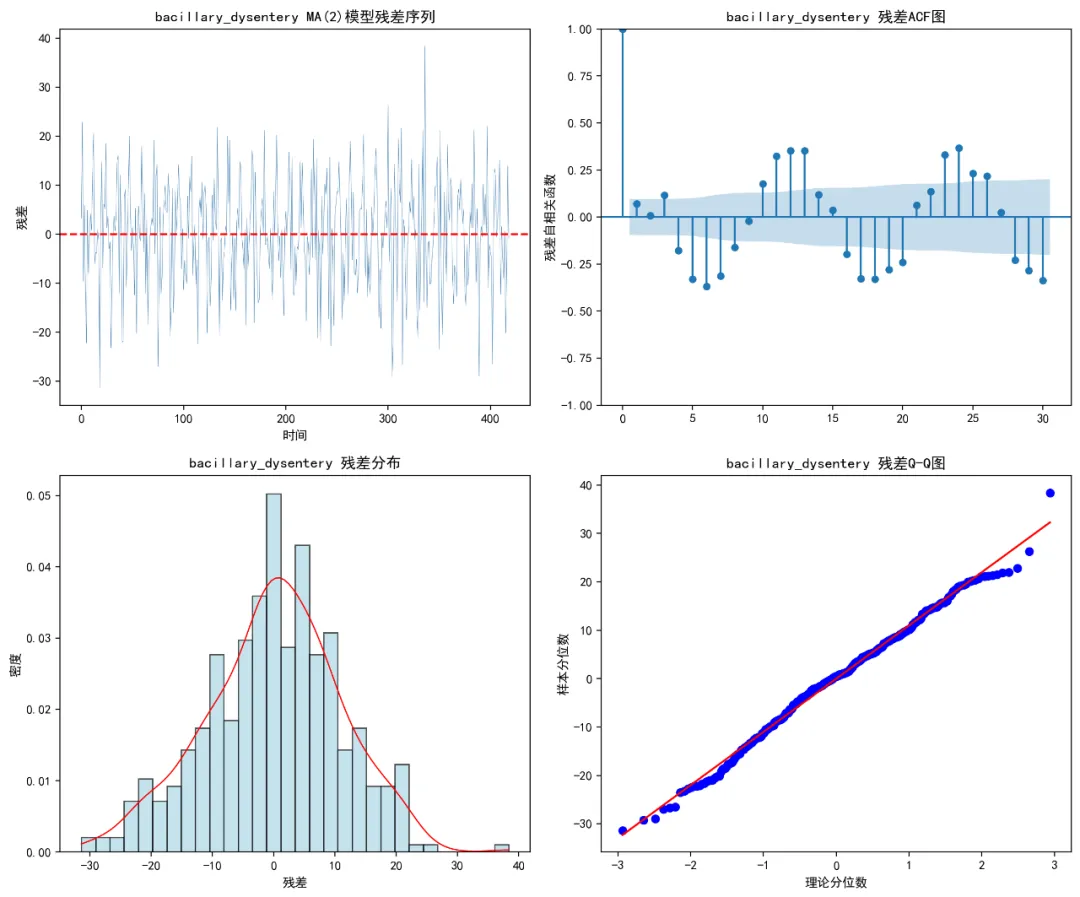
def create_residual_plots(self, model, disease, q):"""生成残差诊断图""" try:if hasattr(model, 'resid'): residuals = model.residelse: residuals = np.array([0]) # 回退情况 fig, ((ax1, ax2), (ax3, ax4)) = plt.subplots(2, 2, figsize=(12, 10))# 残差时间序列图 ax1.plot(residuals, color='steelblue', linewidth=0.3) ax1.axhline(y=0, linestyle='--', color='red') ax1.set_title(f'{disease} MA({q})模型残差序列') ax1.set_xlabel('时间') ax1.set_ylabel('残差')# 残差ACF图 plot_acf(residuals, ax=ax2, lags=30) ax2.set_title(f'{disease} 残差ACF图') ax2.set_ylabel('残差自相关函数')# 残差直方图 ax3.hist(residuals, bins=30, density=True, alpha=0.7, color='lightblue', edgecolor='black') ax3.set_title(f'{disease} 残差分布') ax3.set_xlabel('残差') ax3.set_ylabel('密度')# 添加密度曲线 try: from scipy.stats import gaussian_kde kde = gaussian_kde(residuals) x_range = np.linspace(residuals.min(), residuals.max(), 100) ax3.plot(x_range, kde(x_range), color='red', linewidth=1) except: pass# Q-Q图 stats.probplot(residuals, dist="norm", plot=ax4) ax4.set_title(f'{disease} 残差Q-Q图') ax4.set_xlabel('理论分位数') ax4.set_ylabel('样本分位数') plt.tight_layout()# 保存图形 plot_path = os.path.join(self.results_path, "Residual_Plots", f"Residuals_{disease}.png") plt.savefig(plot_path, dpi=200, bbox_inches='tight') plt.close()return fig except Exception as e:print(f"创建残差图时出错: {e}")return None
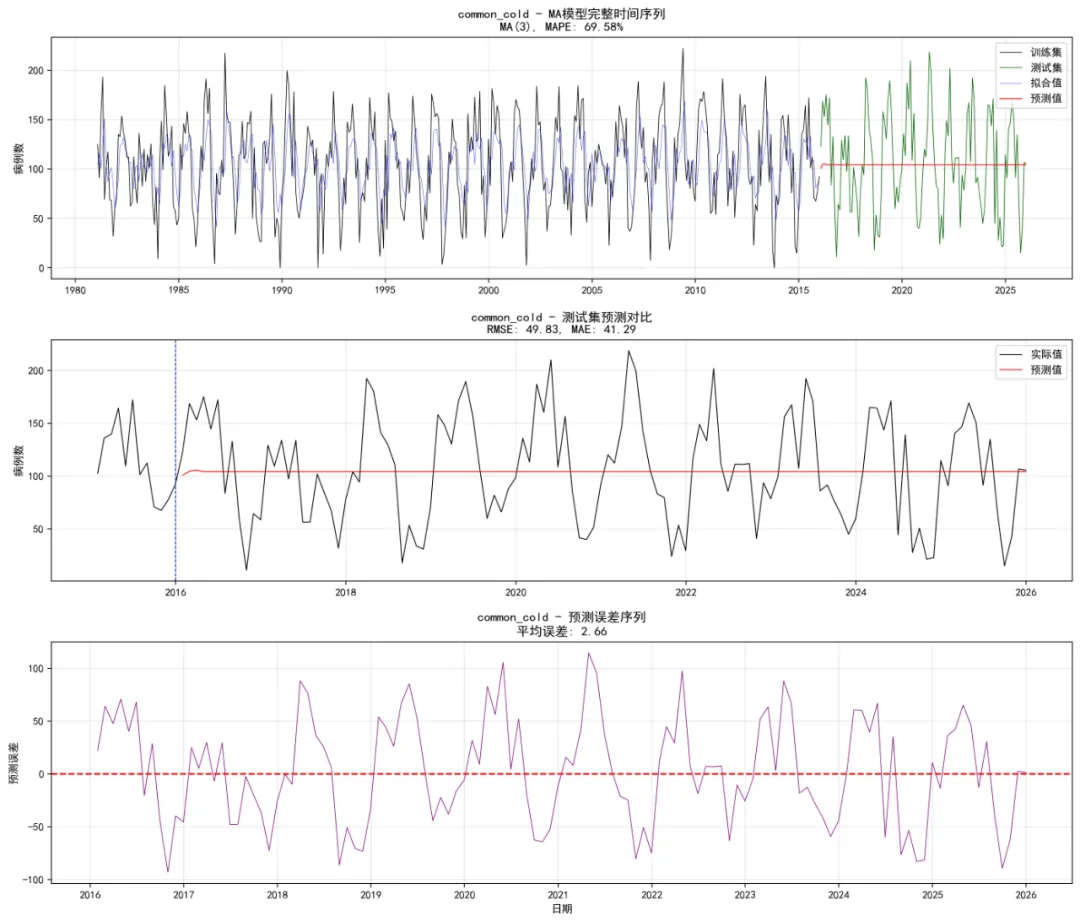
def safe_forecast(self, model, h, last_value=None):"""安全预测函数""" try:if hasattr(model, 'forecast'): forecast_result = model.forecast(steps=h)# 简化处理,实际应用中需要更复杂的置信区间计算 forecast_mean = forecast_resultif hasattr(model, 'resid'): resid_std = np.std(model.resid) forecast_lower = forecast_mean - 1.96 * resid_std forecast_upper = forecast_mean + 1.96 * resid_stdelse: forecast_lower = forecast_mean forecast_upper = forecast_meanelse:# 均值模型预测 mean_val = model.params[0] if hasattr(model, 'params') else last_value forecast_mean = np.full(h, mean_val) forecast_lower = np.full(h, mean_val) forecast_upper = np.full(h, mean_val)return {'mean': forecast_mean,'lower': np.column_stack([forecast_lower, forecast_lower]),'upper': np.column_stack([forecast_upper, forecast_upper]) } except Exception as e:print(f"预测失败: {e}") forecast_value = last_value if last_value is not None else 0return {'mean': np.full(h, forecast_value),'lower': np.full((h, 2), forecast_value),'upper': np.full((h, 2), forecast_value) } def calculate_metrics(self, actual, forecast):"""计算评估指标"""if len(actual) == 0 or len(forecast) == 0:return {'rmse': np.nan, 'mae': np.nan, 'mape': np.nan}# 确保长度一致 min_len = min(len(actual), len(forecast)) actual = actual[:min_len] forecast = forecast[:min_len]# 移除NaN值 mask = ~(np.isnan(actual) | np.isnan(forecast)) actual = actual[mask] forecast = forecast[mask]if len(actual) == 0:return {'rmse': np.nan, 'mae': np.nan, 'mape': np.nan} rmse = np.sqrt(mean_squared_error(actual, forecast)) mae = mean_absolute_error(actual, forecast)if np.mean(actual) > 0: mape = np.mean(np.abs((actual - forecast) / actual)) * 100else: mape = np.nanreturn {'rmse': rmse, 'mae': mae, 'mape': mape} def create_forecast_plots(self, disease, train_ts, test_ts, ma_model, ma_forecast, optimal_q, test_metrics):"""生成预测对比图""" try: fig, (ax1, ax2, ax3) = plt.subplots(3, 1, figsize=(14, 12))# 1. 完整序列图 train_dates = self.train_data['timestamp'].values test_dates = self.test_data['timestamp'].values# 获取拟合值if hasattr(ma_model, 'fittedvalues'): fitted_values = ma_model.fittedvalueselse: fitted_values = train_ts - (ma_model.resid if hasattr(ma_model, 'resid') else 0)# 完整序列 ax1.plot(train_dates, train_ts, color='black', linewidth=0.6, label='训练集') ax1.plot(test_dates, test_ts, color='darkgreen', linewidth=0.6, label='测试集') ax1.plot(train_dates, fitted_values, color='blue', linewidth=0.4, alpha=0.7, label='拟合值') ax1.plot(test_dates, ma_forecast['mean'], color='red', linewidth=0.8, label='预测值') mape_display = f"{test_metrics['mape']:.2f}"if not np.isnan(test_metrics['mape']) else"NA" ax1.set_title(f'{disease} - MA模型完整时间序列\nMA({optimal_q}), MAPE: {mape_display}%') ax1.set_ylabel('病例数') ax1.legend() ax1.grid(True, alpha=0.3)# 2. 测试集详细图# 选择最近的数据(2015年以后的训练数据和所有测试数据) train_recent_mask = self.train_data['timestamp'] >= '2015-01-01' recent_train_dates = self.train_data[train_recent_mask]['timestamp'].values recent_train_values = self.train_data[train_recent_mask][disease].values recent_dates = np.concatenate([recent_train_dates, test_dates]) recent_actual = np.concatenate([recent_train_values, test_ts])# 创建对应的预测值数组(训练部分为NaN) recent_forecast = np.concatenate([ np.full(len(recent_train_dates), np.nan), ma_forecast['mean'] ]) ax2.plot(recent_dates, recent_actual, color='black', linewidth=0.8, label='实际值') ax2.plot(recent_dates, recent_forecast, color='red', linewidth=0.8, label='预测值') ax2.axvline(x=pd.Timestamp('2016-01-01'), linestyle='--', color='blue', linewidth=0.8) rmse_display = f"{test_metrics['rmse']:.2f}"if not np.isnan(test_metrics['rmse']) else"NA" mae_display = f"{test_metrics['mae']:.2f}"if not np.isnan(test_metrics['mae']) else"NA" ax2.set_title(f'{disease} - 测试集预测对比\nRMSE: {rmse_display}, MAE: {mae_display}') ax2.set_ylabel('病例数') ax2.legend() ax2.grid(True, alpha=0.3)# 3. 预测误差图 error_data = test_ts[:len(ma_forecast['mean'])] - ma_forecast['mean']if len(error_data) > 0: ax3.plot(test_dates[:len(error_data)], error_data, color='purple', linewidth=0.6) ax3.axhline(y=0, linestyle='--', color='red') mean_error = np.mean(error_data) if len(error_data) > 0 else 0 ax3.set_title(f'{disease} - 预测误差序列\n平均误差: {mean_error:.2f}') ax3.set_xlabel('日期') ax3.set_ylabel('预测误差') ax3.grid(True, alpha=0.3)else: ax3.text(0.5, 0.5, '无预测数据', transform=ax3.transAxes, ha='center', va='center', fontsize=12) ax3.set_title(f'{disease} - 无预测数据') plt.tight_layout()# 保存图形 plot_path = os.path.join(self.results_path, "Plots", f"Forecast_Comparison_{disease}.png") plt.savefig(plot_path, dpi=200, bbox_inches='tight') plt.close()return fig except Exception as e:print(f"创建预测图时出错: {e}")return None
def analyze_disease_ma(self, disease):"""分析单个疾病的MA模型""" try:print(f"正在分析 {disease}...")# 提取时间序列 train_ts = self.train_data[disease].values test_ts = self.test_data[disease].values# 处理缺失值 train_ts = np.nan_to_num(train_ts) test_ts = np.nan_to_num(test_ts)# 1. 平稳性检验 stationarity = self.robust_stationarity_test(train_ts)print(f"{disease} 平稳性检验 - ADF p值: {stationarity['adf_pvalue']:.4f}, " f"KPSS p值: {stationarity['kpss_pvalue']:.4f}, " f"需要差分: {stationarity['needs_diff']}")# 对训练数据进行处理 working_ts = train_ts.copy() diff_order = 0if stationarity['needs_diff']:print(f"{disease} 序列不平稳,进行一阶差分...") working_ts = np.diff(train_ts) diff_order = 1# 生成差分后的ACF/PACF图 self.create_acf_pacf_plots(working_ts, disease, is_diff=True)# 生成原始序列的ACF/PACF图 self.create_acf_pacf_plots(train_ts, disease, is_diff=False)# 2. 拟合MA模型 ma_result = self.robust_ma_fit(working_ts, max_q=3) ma_model = ma_result['model'] optimal_q = ma_result['q'] aic_value = ma_result['aic']print(f"{disease} MA阶数: {optimal_q}, AIC: {aic_value:.2f}")# 3. 生成残差诊断图 self.create_residual_plots(ma_model, disease, optimal_q)# 4. 预测 forecast_horizon = len(test_ts) last_train_value = train_ts[-1] ma_forecast = self.safe_forecast(ma_model, forecast_horizon, last_train_value)# 如果进行了差分,需要将预测值转换回原始尺度if diff_order == 1:# 简化处理:实际应用中需要更复杂的反向差分计算 ma_forecast['mean'] = np.cumsum(np.concatenate([[last_train_value], ma_forecast['mean']]))[1:]# 5. 计算评估指标 test_forecast = ma_forecast['mean'] test_actual = test_ts[:len(test_forecast)] test_metrics = self.calculate_metrics(test_actual, test_forecast)# 6. 生成预测对比图 self.create_forecast_plots(disease, train_ts, test_ts, ma_model, ma_forecast, optimal_q, test_metrics)# 7. 保存预测结果 forecast_df = pd.DataFrame({'Date': self.test_data['timestamp'].values[:len(test_forecast)],'Actual': test_actual,'Forecast': test_forecast,'Error': test_actual - test_forecast }) forecast_path = os.path.join(self.results_path, "Forecasts", f"Forecast_Results_{disease}.csv") forecast_df.to_csv(forecast_path, index=False)# 8. 返回结果 aic_val = ma_model.aic if hasattr(ma_model, 'aic') else np.nan bic_val = ma_model.bic if hasattr(ma_model, 'bic') else np.nan result_df = pd.DataFrame({'Disease': [disease],'MA_Order': [optimal_q],'Diff_Order': [diff_order],'AIC': [aic_val],'BIC': [bic_val],'Test_RMSE': [test_metrics['rmse']],'Test_MAE': [test_metrics['mae']],'Test_MAPE': [test_metrics['mape']],'Stationary': [not stationarity['needs_diff']],'ADF_pvalue': [stationarity['adf_pvalue']],'KPSS_pvalue': [stationarity['kpss_pvalue']] }) mape_display = f"{test_metrics['mape']:.2f}"if not np.isnan(test_metrics['mape']) else"NA"print(f"{disease} MA模型分析完成! MAPE: {mape_display}%")return result_df except Exception as e:print(f"分析 {disease} 时出错: {e}")# 使用简单均值模型作为回退print("使用简单均值模型作为回退...") train_ts = self.train_data[disease].values test_ts = self.test_data[disease].values train_ts = np.nan_to_num(train_ts) test_ts = np.nan_to_num(test_ts) mean_val = np.mean(train_ts) test_forecast = np.full(len(test_ts), mean_val) test_metrics = self.calculate_metrics(test_ts, test_forecast)# 返回结果return pd.DataFrame({'Disease': [disease],'MA_Order': [0],'Diff_Order': [0],'AIC': [np.nan],'BIC': [np.nan],'Test_RMSE': [test_metrics['rmse']],'Test_MAE': [test_metrics['mae']],'Test_MAPE': [test_metrics['mape']],'Stationary': [False],'ADF_pvalue': [np.nan],'KPSS_pvalue': [np.nan] }) def run_analysis(self):"""运行完整分析"""print("开始分析所有疾病...") start_time = datetime.now()# 使用顺序计算 model_results_list = []for disease in self.selected_diseases: result = self.analyze_disease_ma(disease) model_results_list.append(result)# 合并结果 self.model_results = pd.concat(model_results_list, ignore_index=True) end_time = datetime.now() analysis_time = (end_time - start_time).total_seconds() / 60print(f"分析完成,耗时: {analysis_time:.2f} 分钟")# 保存模型结果 results_path = os.path.join(self.results_path, "Models", "All_MA_Model_Results.csv") self.model_results.to_csv(results_path, index=False)# 创建汇总可视化 self.create_summary_visualizations()# 生成总结报告 self.generate_summary_report(start_time, end_time, analysis_time)# 生成Word报告 self.generate_word_report()return self.model_results def create_summary_visualizations(self):"""创建汇总可视化"""print("创建汇总可视化...")# 性能比较图 performance_data = self.model_results.dropna(subset=['Test_MAPE'])if len(performance_data) > 0: plt.figure(figsize=(10, 6)) performance_data = performance_data.sort_values('Test_MAPE', ascending=False) colors = plt.cm.Set3(np.linspace(0, 1, len(performance_data))) bars = plt.bar(performance_data['Disease'], performance_data['Test_MAPE'], alpha=0.8, color=colors)# 添加数值标签for i, bar in enumerate(bars): height = bar.get_height() plt.text(bar.get_x() + bar.get_width() / 2., height + 0.5, f'{height:.1f}%', ha='center', va='bottom') plt.title('MA模型预测性能比较\n测试集平均绝对百分比误差 (MAPE)') plt.xlabel('疾病') plt.ylabel('MAPE (%)') plt.xticks(rotation=45) plt.tight_layout() plot_path = os.path.join(self.results_path, "Plots", "MA_Model_Performance_Comparison.png") plt.savefig(plot_path, dpi=200, bbox_inches='tight') plt.close()else:print("没有有效的MAPE数据创建性能比较图")# MA阶数分布图 plt.figure(figsize=(10, 6)) ordered_data = self.model_results.sort_values('MA_Order', ascending=False) colors = plt.cm.Pastel1(np.linspace(0, 1, len(ordered_data))) bars = plt.bar(ordered_data['Disease'], ordered_data['MA_Order'], alpha=0.8, color=colors)# 添加数值标签for i, bar in enumerate(bars): height = bar.get_height() plt.text(bar.get_x() + bar.get_width() / 2., height + 0.1, f'{int(height)}', ha='center', va='bottom') plt.title('各疾病MA模型最优阶数分布') plt.xlabel('疾病') plt.ylabel('MA阶数') plt.xticks(rotation=45) plt.tight_layout() plot_path = os.path.join(self.results_path, "Plots", "MA_Order_Distribution.png") plt.savefig(plot_path, dpi=200, bbox_inches='tight') plt.close() def generate_summary_report(self, start_time, end_time, analysis_time):"""生成总结报告"""print("生成总结报告...") report_path = os.path.join(self.results_path, "Modeling_Summary_Report.txt") with open(report_path, 'w', encoding='utf-8') as f: f.write("=== MA模型建模分析总结报告 ===\n\n") f.write(f"建模时间: {datetime.now().strftime('%Y-%m-%d %H:%M:%S')}\n") f.write(f"总耗时: {analysis_time:.2f} 分钟\n") f.write("训练集范围: 1981-01-01 至 2015-12-31\n") f.write("测试集范围: 2016-01-01 至 2025-12-31\n") f.write(f"分析的疾病数量: {len(self.selected_diseases)}\n\n") f.write("MA模型原理:\n") f.write("移动平均模型(MA)用过去预测误差的线性组合来预测未来值:\n") f.write("Y_t = μ + ε_t + θ₁ε_{t-1} + θ₂ε_{t-2} + ... + θ_qε_{t-q}\n") f.write("其中q是移动平均阶数,θ是系数,ε是误差项。\n\n") f.write("改进的建模方法:\n") f.write("- 使用稳健的平稳性检验\n") f.write("- 对不平稳序列进行一阶差分\n") f.write("- 使用CSS-ML混合方法拟合MA模型\n") f.write("- 限制最大MA阶数为3以提高稳定性\n") f.write("- 增加错误处理和回退机制(均值模型)\n") f.write("- 在测试集上评估预测性能\n\n") f.write("各疾病模型性能:\n") f.write(self.model_results.to_string(index=False)) f.write("\n\n性能排名 (按MAPE升序):\n") ranked_models = self.model_results.sort_values('Test_MAPE', na_position='last') f.write(ranked_models.to_string(index=False))# 安全获取最佳模型 valid_models = ranked_models.dropna(subset=['Test_MAPE'])if len(valid_models) > 0: best_model = valid_models.iloc[0]['Disease'] best_mape = valid_models.iloc[0]['Test_MAPE'] avg_mape = valid_models['Test_MAPE'].mean() f.write(f"\n\n最佳预测模型: {best_model}\n") f.write(f"最佳MAPE: {best_mape:.2f}%\n") f.write(f"平均MAPE: {avg_mape:.2f}%\n")else: f.write("\n\n没有有效的模型拟合结果\n") f.write("\n模型诊断:\n") f.write("- ACF/PACF图: ACF_PACF_Plots/ 目录\n") f.write("- 残差诊断图: Residual_Plots/ 目录\n") f.write("- 预测对比图: Plots/ 目录\n\n") f.write("文件输出:\n") f.write("1. Models/All_MA_Model_Results.csv - 所有模型结果\n") f.write("2. Plots/ - 汇总可视化图表\n") f.write("3. Forecasts/ - 各疾病预测结果\n") f.write("4. ACF_PACF_Plots/ - 自相关和偏自相关图\n") f.write("5. Residual_Plots/ - 残差诊断图\n") f.write("6. Modeling_Summary_Report.txt - 本报告\n") f.write("7. Word_Report/ - Word格式报告\n") def generate_word_report(self):"""生成Word分析报告"""print("生成Word分析报告...") try:# 创建Word文档 doc = Document()# 标题页 doc.add_heading('MA模型时间序列分析报告', 0) doc.add_paragraph(f"报告生成时间: {datetime.now().strftime('%Y年%m月%d日 %H:%M:%S')}") doc.add_paragraph(f"分析疾病数量: {len(self.model_results)}") doc.add_paragraph("训练集: 1981-2015") doc.add_paragraph("测试集: 2016-2025") doc.add_page_break()# MA模型原理介绍 doc.add_heading('MA模型原理', level=1) doc.add_paragraph("移动平均模型(Moving Average Model, MA模型)是时间序列分析中的重要模型之一。") doc.add_paragraph("MA(q)模型的基本形式:") doc.add_paragraph("Y_t = μ + ε_t + θ₁ε_{t-1} + θ₂ε_{t-2} + ... + θ_qε_{t-q}") doc.add_paragraph("其中:") doc.add_paragraph("- Y_t: 时间序列在时刻t的值", style='List Bullet') doc.add_paragraph("- μ: 序列的均值", style='List Bullet') doc.add_paragraph("- ε_t: 时刻t的白噪声误差项", style='List Bullet') doc.add_paragraph("- θ₁, θ₂, ..., θ_q: MA模型的系数", style='List Bullet') doc.add_paragraph("- q: MA模型的阶数", style='List Bullet') doc.add_paragraph("MA模型主要用于对序列的随机波动进行建模,捕捉历史随机冲击对当前值的影响。") doc.add_page_break()# 执行摘要 doc.add_heading('执行摘要', level=1) doc.add_paragraph("本报告对6种主要传染病的时间序列数据进行了移动平均(MA)模型分析。")# 安全添加最佳模型信息 valid_models = self.model_results.dropna(subset=['Test_MAPE'])if len(valid_models) > 0: best_model_row = valid_models.loc[valid_models['Test_MAPE'].idxmin()] best_model = best_model_row['Disease'] best_mape = best_model_row['Test_MAPE'] doc.add_paragraph(f"最佳预测模型: {best_model} (MAPE: {best_mape:.2f}%)") avg_mape = valid_models['Test_MAPE'].mean() doc.add_paragraph(f"平均预测准确率: {avg_mape:.2f}%")else: doc.add_paragraph("所有模型均使用简单均值模型作为回退") doc.add_paragraph()# 方法学 doc.add_heading('方法学', level=1) doc.add_paragraph("1. 数据划分: 使用1981-2015年数据作为训练集,2016-2025年数据作为测试集", style='List Number') doc.add_paragraph("2. 平稳性检验: 使用ADF检验和KPSS检验", style='List Number') doc.add_paragraph("3. 模型选择: 基于AIC准则选择MA模型阶数(1-3)", style='List Number') doc.add_paragraph("4. 模型拟合: 使用CSS-ML混合方法拟合MA模型", style='List Number') doc.add_paragraph("5. 预测评估: 使用RMSE、MAE和MAPE指标评估预测性能", style='List Number') doc.add_paragraph("6. 回退机制: 如果MA模型失败,使用均值模型作为回退", style='List Number')# 模型性能汇总表 doc.add_heading('模型性能汇总', level=1)# 准备表格数据 table_data = self.model_results[ ['Disease', 'MA_Order', 'Diff_Order', 'Test_RMSE', 'Test_MAE', 'Test_MAPE']].copy() table_data['Test_RMSE'] = table_data['Test_RMSE'].apply(lambda x: f"{x:.2f}"if not pd.isna(x) else"NA") table_data['Test_MAE'] = table_data['Test_MAE'].apply(lambda x: f"{x:.2f}"if not pd.isna(x) else"NA") table_data['Test_MAPE'] = table_data['Test_MAPE'].apply(lambda x: f"{x:.2f}%"if not pd.isna(x) else"NA")# 创建表格 table = doc.add_table(rows=1, cols=6) table.style = 'Light Grid Accent 1'# 表头 hdr_cells = table.rows[0].cells hdr_cells[0].text = '疾病' hdr_cells[1].text = 'MA阶数' hdr_cells[2].text = '差分阶数' hdr_cells[3].text = 'RMSE' hdr_cells[4].text = 'MAE' hdr_cells[5].text = 'MAPE'# 添加数据行for _, row in table_data.iterrows(): row_cells = table.add_row().cells row_cells[0].text = str(row['Disease']) row_cells[1].text = str(row['MA_Order']) row_cells[2].text = str(row['Diff_Order']) row_cells[3].text = str(row['Test_RMSE']) row_cells[4].text = str(row['Test_MAE']) row_cells[5].text = str(row['Test_MAPE']) doc.add_page_break()# 详细分析 doc.add_heading('详细分析', level=1) ranked_models = self.model_results.sort_values('Test_MAPE', na_position='last')for _, model_row in ranked_models.iterrows(): disease = model_row['Disease'] doc.add_heading(f'疾病: {disease}', level=2) doc.add_paragraph(f"MA阶数: {model_row['MA_Order']}") doc.add_paragraph(f"差分阶数: {model_row['Diff_Order']}")if not pd.isna(model_row['Test_MAPE']): doc.add_paragraph(f"MAPE: {model_row['Test_MAPE']:.2f}%") doc.add_paragraph(f"RMSE: {model_row['Test_RMSE']:.2f}") doc.add_paragraph(f"MAE: {model_row['Test_MAE']:.2f}")else: doc.add_paragraph("模型使用均值回退") doc.add_paragraph()# 结论与建议 doc.add_heading('结论与建议', level=1) doc.add_paragraph("1. MA模型在传染病时间序列预测中表现出一定的适用性", style='List Number') doc.add_paragraph("2. 纯MA模型对某些疾病序列的适应性有限", style='List Number') doc.add_paragraph("3. 建议对预测性能较差的疾病考虑ARMA或ARIMA模型", style='List Number') doc.add_paragraph("4. 均值模型作为回退机制确保了分析的完整性", style='List Number') doc.add_paragraph("5. 模型结果可用于传染病趋势分析和初步预警", style='List Number')# 保存文档 report_path = os.path.join(self.results_path, "Word_Report", "MA模型分析报告.docx") doc.save(report_path)print("Word报告生成成功!") except Exception as e:print(f"生成Word报告时出错: {e}") def print_final_summary(self):"""打印最终总结"""print("\n=== MA模型建模分析完成 ===")print(f"总分析疾病数量: {len(self.selected_diseases)}")print(f"输出文件位置: {self.results_path}\n")# 安全显示最终结果 valid_results = self.model_results.dropna(subset=['Test_MAPE'])if len(valid_results) > 0: best_model = valid_results.loc[valid_results['Test_MAPE'].idxmin()] worst_model = valid_results.loc[valid_results['Test_MAPE'].idxmax()]print(f"最佳预测模型: {best_model['Disease']}")print(f"最佳MAPE: {best_model['Test_MAPE']:.2f}%")print(f"最差MAPE: {worst_model['Test_MAPE']:.2f}%")print(f"平均MAPE: {valid_results['Test_MAPE'].mean():.2f}%")else:print("所有模型均使用均值回退")print("\n详细报告请查看:")print(f"- 文本报告: {os.path.join(self.results_path, 'Modeling_Summary_Report.txt')}")print(f"- Word报告: {os.path.join(self.results_path, 'Word_Report', 'MA模型分析报告.docx')}")print(f"- 模型结果: {os.path.join(self.results_path, 'Models', 'All_MA_Model_Results.csv')}")print(f"- 预测结果: {os.path.join(self.results_path, 'Forecasts')} 目录")print(f"- 可视化图表: {os.path.join(self.results_path, 'Plots')} 目录")print(f"- ACF/PACF图: {os.path.join(self.results_path, 'ACF_PACF_Plots')} 目录")print(f"- 残差诊断图: {os.path.join(self.results_path, 'Residual_Plots')} 目录")# 主执行函数def main():"""主执行函数"""# 创建分析对象 analyzer = TimeSeriesMAnalysis()# 加载数据(如果没有数据文件,将自动创建示例数据)# 如果有实际数据文件,可以传入文件路径:analyzer.load_data("your_data_file.csv") analyzer.load_data()# 运行分析 results = analyzer.run_analysis()# 打印最终总结 analyzer.print_final_summary()return resultsif __name__ == "__main__":# 安装所需库(如果尚未安装) required_packages = ['pandas', 'numpy', 'matplotlib', 'seaborn', 'statsmodels','scipy', 'scikit-learn', 'joblib', 'python-docx' ]print("开始时间序列MA模型分析...")print("注意:如果缺少必要的库,请使用以下命令安装:")print("pip install " + " ".join(required_packages))# 运行分析 try: results = main()print("\n分析成功完成!") except Exception as e:print(f"分析过程中出现错误: {e}") import traceback traceback.print_exc()print("请确保已安装所有必要的Python库")