用 Python 和 Streamlit 求解

马科维茨有效前沿

在本篇文章，我们将探讨每位经济学专业学生在大学毕业前都应掌握的技能。

这篇文章将带你一步步使用 Python 和 Streamlit 求解马科维茨（Markowitz）的有效前沿（Efficient Frontier）。

第一部分，我们将探索如何通过模拟来优化投资组合配置；第二部分，我们将涵盖交易策略的回测，以评估马科维茨理论的实际适用性。我们的主要目标是判断是否因风险变化而需要对投资组合进行再平衡。

有效前沿

有效前沿（Efficient Frontier, EF）理论由诺贝尔奖得主哈里·马科维茨（Harry Markowitz）于1952年提出，是现代投资组合理论（Modern Portfolio Theory, MPT）的核心概念。复合年增长率（CAGR）代表收益，而年化标准差则表示风险。相关的基本概念在大学金融学专业本科核心课程金融学、投资学、投资组合管理中会学到。

有效前沿以图形方式展示那些在给定风险水平下能实现最大收益的投资组合。投资者的目标是构建高收益、低整体风险的投资组合。该理论依赖于资产之间的协方差。

均值-方差优化（Mean-Variance Optimization, MVO）

MVO 是一种优化技术，用于确定投资组合中各资产的权重，以在更低风险下实现更高收益。它依赖历史数据来估计预期收益和协方差矩阵。MVO 假设投资者仅基于预期收益和风险做出决策，忽略了税收、交易成本、流动性、技术分析和基本面分析等其他因素。因此，它也忽视了诸如内幕交易之类的非对称信息。

MVO 不区分正向风险与负向风险。由于投资者通常具有风险厌恶倾向，他们可能更关注避免负收益，而非捕捉潜在的正收益。这也是我们应用这个理论需要特别注意的一点。正如牛市冲顶、熊市下探，投资者更倾向于担忧市场回调，而非享受收益上涨。

夏普比率（Sharpe Ratio）

为了获得最优配置的投资组合，我们必须定义三个基本变量：

Rp  = 投资组合的预期收益Rf  = 无风险收益率StdDev(Rp) = 投资组合收益的标准差

预期投资组合收益通常通过历史经验数据计算得出，一般采用每日对数收益率的平均值。为将其年化，通常按 252 个交易日进行换算。

由于预期收益和标准差均由历史市场数据决定，因此假设它们在未来保持不变是一个重大前提。这正是现代投资组合理论（MPT）的一个关键弱点，因为大多数时间序列都被认为是非平稳的随机过程。

我们利用上述变量计算夏普比率，夏普比率为 1 表示风险与预期收益达到均衡：

投资组合通常以最大化夏普比率为优化目标。

配置 Streamlit

streamlit有session的概念，如何使用参见streamlit文档。举个简单例子：

import streamlit as stimport pandas as pdclass SessionState:    def __init__(self, **kwargs):        for key, val in kwargs.items():            setattr(self, key, val)@st.cache(allow_output_mutation=True)def get_session():    return SessionState(df=pd.DataFrame())session_state = get_session()# Creating a dictionary with some datadata = {    'Name': ['John', 'Anna', 'Peter', 'Linda'],    'Age': [28, 35, 40, 25]}# Creating a DataFrame with the datadf = pd.DataFrame(data)# Assigning this DataFrame to session_statesession_state.df = df

这段代码定义了 SessionState 类，使我们能够将 Python 对象存储在其中。通过调用 get_session 函数，我们可以检索会话状态中保存的任何 Python 对象。

在行动之前你需要安装这些包：

import streamlit as st  # library for building interactive web appsimport pandas as pdimport numpy as npfrom datetime import dateimport requestsfrom io import BytesIOimport yfinance as yfimport base64  # Encoding and decoding binary data to/from ASCIIimport plotly.express as pximport plotly.graph_objects as go 

如果你想从git ub加载一些代码过来，可以这样：

def load_data_from_github(url):    response = requests.get(url)    content = BytesIO(response.content)    data = pd.read_pickle(content)    return data

为方便起见，我们使用 yfinance 库从股票市场获取数据。

def download_data(data, period='1y'):    dfs = []    if isinstance(data, dict):        for name, ticker in data.items():            ticker_obj = yf.Ticker(ticker)            hist = ticker_obj.history(period=period) # timeframe            hist.columns = [f"{name}_{col}" for col in hist.columns]  # Add prefix to the name            hist.index = pd.to_datetime(hist.index.map(lambda x: x.strftime('%Y-%m-%d')))            dfs.append(hist)    elif isinstance(data, list):        for ticker in data:            ticker_obj = yf.Ticker(ticker)            hist = ticker_obj.history(period=period)            hist.columns = [f'{ticker}_{col}' for col in hist.columns]  # Add prefix to the name            hist.index = pd.to_datetime(hist.index.map(lambda x: x.strftime('%Y-%m-%d')))            dfs.append(hist)      combined_df = pd.concat(dfs, axis=1, join='outer')  # Use join='outer' to handle different data indices    return combined_df

用于选择资产的 Streamlit 代码假设你已经定义并存储了一个包含股票代码组合的DataFrame。

这些数据包括开盘价、收盘价、最高价、最低价以及调整后价格。我们使用“调整后收盘价”这一列。

我们构建了四个字典，分别包含 B3 BOVESPA、标普500（S&P500）、纳斯达克、大宗商品、加密货币以及美元（USD）货币对的股票代码。

允许用户选择数据的时间范围，重采样（resampling）、缺失值处理（missing values treatment）和滚动平均值（rolling average），这些功能没有写明具体代码，你keyi根据自己的需求实现。

# select box widget to choose timeframesselected_timeframes = st.selectbox('Select Timeframe:', ['1d', '5d', '1mo', '3mo', '6mo', '1y', '2y', '5y', '10y', 'ytd', 'max'], index=7)# creating a dictionary of dictionaries with all available tickersassets_list = {'CURRENCIES': currencies_dict, 'CRYPTO': crypto_dict, 'B3_STOCKS': b3_stocks, 'SP500': sp500_dict, 'NASDAQ100': nasdaq_dict, 'indexes': indexes_dict}# combining dictionaries when the user selects one or more in assets_listselected_dict_names = st.multiselect('Select dictionaries to combine', list(assets_list.keys()))combined_dict = {}for name in selected_dict_names:    dictionary = assets_list.get(name)    if dictionary:        combined_dict.update(dictionary)# dictionary to actually store retrieved dataselected_ticker_dict = {}# looping through the chosen tickersif selected_dict_names:    # the list to iterate over tickers    tickers = st.multiselect('Asset Selection', list(combined_dict.keys()))    if tickers and st.button("Download data"):        for key in tickers:            if key in combined_dict:                selected_ticker_dict[key] = combined_dict[key]        # Assigning data object as the result of the function download_data        session_state.data = download_data(selected_ticker_dict, selected_timeframes)# Handle tickers entered manuallytype_tickers = st.text_input('Enter Tickers (comma-separated):')if type_tickers and st.button("Download data"):    tickers = [ticker.strip() for ticker in type_tickers.split(',')]    # doing the same for tickers separated by commas    session_state.data = download_data(tickers, selected_timeframes)

如果这些代码成功运行，你将获得一个交互的界面（图传不上去），可以选择股票并下载他们的数据。

生成有效前沿

你也可以用 pyportfolioopt 来完成这项任务。参考Damian Boh, Easily Optimize a Stock Portfolio using PyPortfolioOpt in Python这篇文章。

from pypfopt.efficient_frontier import EfficientFrontierfrom pypfopt import risk_modelsfrom pypfopt import expected_returnsimport pandas as pd# Sample stock data (replace it with Close prices downloaded from yahoo finance)stock_data = {    "AAPL": [0.1, 0.05, 0.08, 0.12, 0.07],    "GOOG": [0.05, 0.06, 0.07, 0.08, 0.09],    "MSFT": [0.06, 0.04, 0.08, 0.07, 0.05]}stocks_df = pd.DataFrame(stock_data)# Calculate expected returns and sample covariance matrixmu = expected_returns.mean_historical_return(stocks_df)S = risk_models.sample_cov(stocks_df)# Create the Efficient Frontier objectef = EfficientFrontier(mu, S)# Optimize for maximum Sharpe ratioweights = ef.max_sharpe()# Clean the weights (optional)cleaned_weights = ef.clean_weights()# Print the cleaned weightsprint(cleaned_weights)# Plot the efficient frontieref.portfolio_performance(verbose=True)

也可以使用求解器（solver）实现最小化（minimize）。这节省大量时间：

• • 估算资产的年化收益率；
• • 计算投资组合的方差；
• • 计算投资组合中每对资产之间的协方差；
• • 计算夏普比率，并确定使该比率最大化的各资产最优权重。
• • 至少需要满足以下约束条件：权重之和必须等于 1，且每个权重必须大于 0（不允许做空）。

import numpy as npimport cvxpy as cp# Risk-free raterisk_free_rate = 0.05# Number of assetsn_assets = len(expected_returns)# Define variablesweights = cp.Variable(n_assets)# Portfolio expected returnportfolio_return = expected_returns @ weights# Portfolio volatility (standard deviation)portfolio_volatility = cp.sqrt(cp.quad_form(weights, covariance_matrix))# Portfolio Sharpe Ratioportfolio_sharpe_ratio = (portfolio_return - risk_free_rate) / portfolio_volatility# Define objective function (maximize Sharpe Ratio)objective = cp.Maximize(portfolio_sharpe_ratio)# Define constraintsconstraints = [    cp.sum(weights) == 1,  # sum of weights equals 1 (fully invested)    weights >= 0  # weights are non-negative]# You can add more constraints here, such as minimum and maximum weights,# target return, etc.# Solve the optimization problemproblem = cp.Problem(objective, constraints)problem.solve()

我们将收益率定义为：明日调整后收盘价与今日调整后收盘价之比的对数。

def logreturns(df):    # Separating the close price in this case    df.columns = df.columns.str.split('_').str[0]    log_returns = np.log(df)    log_returns = df.iloc[:, 0:].pct_change()    fig = px.line(log_returns, x=log_returns.index, y=log_returns.columns[0:].split('_')[0],                  labels={'value': 'log'},                  title='Log Returns')    fig.update_layout(legend_title_text='Assets')    st.plotly_chart(fig)    return log_returns

对数变换使时间序列更平稳。我们可以通过应用增强型迪基-富勒检验（Augmented Dickey-Fuller test）来验证。

仅凭对数收益率本身，很难判断这些资产究竟呈现正收益还是负收益。我们可以从初始日期开始绘制累计收益：将第一个日期设为基准点，迭代计算。

def return_over_time(df):    return_df = pd.DataFrame()    df.columns = df.columns.str.split('_').str[0]    for col in df.columns:        return_df[col] = df[col] / df[col].iloc[0] -1    fig = px.line(return_df, x=return_df.index, y=return_df.columns[0:],                  labels={'value': 'Returns to Date'},                  title='returns')    fig.update_layout(legend_title_text='Assets')    st.plotly_chart(fig) # for streamlit plots

投资组合的收益

计算投资组合收益需要将权重与平均对数收益率相乘。尽管每次模拟中权重是随机生成的，但平均对数收益率要求我们假设数据的均值。

在此情况下，我们遵循以下步骤：

• • 根据所选时间范围对数据框进行重采样
• • 计算这些收益率的平均值
• • 乘以交易天数（通常为252天），以获得年化收益率

resampler = 'A'  # for annualtrading_days = 252  # usual trading year# Step 1. Resample keeping only the last values of each yearannualized_returns = df.resample(resampler).last()# Step 2. Calculate the log returns and take the average# Step 3. Multiply it by trading daysannualized_returns = df.pct_change().apply(lambda x: np.log(1 + x)).mean() * trading_dayssimple_returns = np.exp(annualized_returns) - 1

你可以根据需要对重采样后的投资组合进行年化处理。例如，如果你希望进行季度分析，只需将重采样参数改为 '3M' 。由于均值-方差优化（Mean-Variance Optimization, MVO）假设收益服从正态分布，因此年化收益是标准做法。

一种更为保守的方法是：不对原始数据框进行重采样，直接计算每日对数收益率的平均值，然后乘以交易天数。一般来讲，夏普比率确实对你计算平均收益的方式非常敏感，这意味着“截至今日的收益在未来可被复制”这一隐含假设不成立。

投资组合收益可以通过将每项资产的收益与其权重相乘后求和得到：

计算资产组合收益方差：

trading_days = 252var = cov_matrix.mul(weights, axis=0).mul(weights, axis=1).sum().sum()sd = np.sqrt(var) # obtain the risk ann_sd = sd*np.sqrt(trading_days) # to scale the risk for any timeframe

模拟有效前沿：

def efficient_frontier(df,                        trading_days,                        risk_free_rate,                       simulations= 1000,                        resampler='A'):    # covariance matrix of the log returns    cov_matrix = df.pct_change().apply(lambda x: np.log(1+x)).cov()    # lists to store the results    portfolio_returns = []     portfolio_variance = []     portfolio_weights = []     num_assets = len(df.columns)    for _ in range(simulations):        # generating up to 1000 portfolio simulations        weights = np.random.random(num_assets)        weights = weights/np.sum(weights) # scaling weights to 1        portfolio_weights.append(weights)        # calculating the log returns        returns = df.resample(resampler).last()        returns = df.pct_change().apply(lambda x: np.log(1 + x)).mean() * trading_days        annualized_returns = np.dot(weights, returns)        portfolio_returns.append(annualized_returns)        # portfolio variance        var = cov_matrix.mul(weights, axis=0).mul(weights, axis=1).sum().sum()        sd = np.sqrt(var) # Daily standard deviation        ann_sd = sd*np.sqrt(trading_days)        portfolio_variance.append(ann_sd)        # storing returns and volatitly in a dataframe        data = {'Returns':portfolio_returns, 'Volatility':portfolio_variance}    for counter, symbol in enumerate(df.columns.tolist()):        data[symbol+' weight'] = [w[counter] for w in portfolio_weights]    simulated_portfolios  = pd.DataFrame(data)    simulated_portfolios['Sharpe_ratio'] = (simulated_portfolios['Returns'] - risk_free_rate) / simulated_portfolios['Volatility']    return simulated_portfolios    

画出有效前沿：

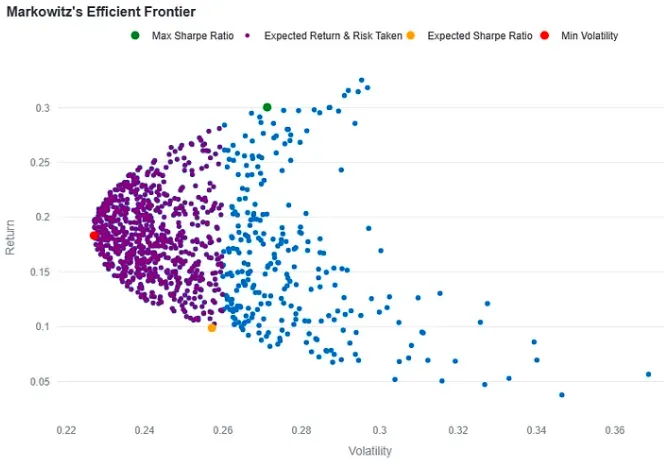
def plot_efficient_frontier(simulated_portfolios, expected_sharpe, expected_return, risk_taken):    simulated_portfolios = simulated_portfolios.sort_values(by='Volatility')    # concatenating weights so we can hover on them as we select data points    simulated_portfolios['Weights'] = simulated_portfolios.iloc[:, 2:-1].apply(        lambda row: ', '.join([f'{asset}: {weight:.4f}' for asset, weight in zip(simulated_portfolios.columns[2:-1], row)]),        axis=1    )    # creating the plot as a scatter graph    frontier = px.scatter(simulated_portfolios, x='Volatility', y='Returns', width=800, height=600,                           title="Markowitz's Efficient Frontier", labels={'Volatility': 'Volatility', 'Returns': 'Return'},                          hover_name='Weights')    # getting the index of max Sharpe Ratio and painting in green    max_sharpe_ratio_portfolio = simulated_portfolios.loc[simulated_portfolios['Sharpe_ratio'].idxmax()]    frontier.add_trace(go.Scatter(x=[max_sharpe_ratio_portfolio['Volatility']],                                   y=[max_sharpe_ratio_portfolio['Returns']],                                  mode='markers',                                  marker=dict(color='green', size=10),                                  name='Max Sharpe Ratio',                                  text=max_sharpe_ratio_portfolio['Weights']))    # Getting portfolios where returns are above our expectations and below     # the amount of risk we aim to take    low_risk_portfolios = simulated_portfolios[        (simulated_portfolios['Returns'] >= expected_return) &         (simulated_portfolios['Volatility'] <= risk_taken)    ]    frontier.add_trace(go.Scatter(x=low_risk_portfolios['Volatility'],                                   y=low_risk_portfolios['Returns'],                                  mode='markers',                                  marker=dict(color='purple', size=5),                                  name='Expected Return & Risk Taken',                                  text=low_risk_portfolios['Weights']))    # Selecting portfolios with our initial Sharpe ratio expectations    # and paiting it orange    expected_portfolio = simulated_portfolios[        (simulated_portfolios['Sharpe_ratio'] >= expected_sharpe - 0.001) &         (simulated_portfolios['Sharpe_ratio'] <= expected_sharpe + 0.001)    ]    if not expected_portfolio.empty:        frontier.add_trace(go.Scatter(x=[expected_portfolio['Volatility'].values[0]],                                       y=[expected_portfolio['Returns'].values[0]],                                      mode='markers',                                      marker=dict(color='orange', size=10),                                      name='Expected Sharpe Ratio',                                      text=expected_portfolio['Weights']))    # selecting the portfolio with lowest risk and painting it red    frontier.add_trace(go.Scatter(x=[simulated_portfolios.iloc[0]['Volatility']],                                   y=[simulated_portfolios.iloc[0]['Returns']],                                  mode='markers',                                  marker=dict(color='red', size=10),                                  name='Min Volatility',                                   text=simulated_portfolios.iloc[0]['Weights']))    frontier.update_layout(legend=dict(                           orientation='h',                           yanchor='top',                           y=1.1,                           xanchor='center',                           x=0.5))    st.plotly_chart(frontier)

大概长这样：