数学建模与Python:能量模拟-从分子运动到宏观热力学

import numpy as npimport matplotlib.pyplot as pltfrom matplotlib.animation import FuncAnimation# 理想气体分子动力学模拟# 1. 系统参数N = 200# 分子数量BOX_SIZE = 10.0# 容器边长V_MAX = 2.0# 最大初始速度MASS = 1.0# 分子质量RADIUS = 0.1# 分子半径DT = 0.05# 时间步长STEPS = 500# 模拟步数# 2. 初始化状态# 随机位置 (避开边界)pos = np.random.uniform(RADIUS, BOX_SIZE - RADIUS, size=(N, 2))# 随机速度vel = np.random.uniform(-V_MAX, V_MAX, size=(N, 2))# 存储历史数据用于绘图history = {'pos': [], 'ke': [], 'pressure': []}# 3. 模拟循环defstep(pos, vel):# 更新位置    pos += vel * DT    # 碰撞检测：与墙壁碰撞 (弹性碰撞)# x 方向边界    mask_x_left = pos[:, 0] < RADIUS    mask_x_right = pos[:, 0] > BOX_SIZE - RADIUS    # 动量变化用于计算压力 (F = dp/dt)    impulse = 0.0if np.any(mask_x_left):        pos[mask_x_left, 0] = RADIUS        vel[mask_x_left, 0] *= -1        impulse += np.sum(2 * MASS * np.abs(vel[mask_x_left, 0]))        if np.any(mask_x_right):        pos[mask_x_right, 0] = BOX_SIZE - RADIUS        vel[mask_x_right, 0] *= -1        impulse += np.sum(2 * MASS * np.abs(vel[mask_x_right, 0]))        # y 方向边界    mask_y_bottom = pos[:, 1] < RADIUS    mask_y_top = pos[:, 1] > BOX_SIZE - RADIUS    if np.any(mask_y_bottom):        pos[mask_y_bottom, 1] = RADIUS        vel[mask_y_bottom, 1] *= -1        impulse += np.sum(2 * MASS * np.abs(vel[mask_y_bottom, 1]))        if np.any(mask_y_top):        pos[mask_y_top, 1] = BOX_SIZE - RADIUS        vel[mask_y_top, 1] *= -1        impulse += np.sum(2 * MASS * np.abs(vel[mask_y_top, 1]))        # 计算瞬时动能 (内能)# KE = 0.5 * m * v^2    ke = 0.5 * MASS * np.sum(vel**2)    # 计算瞬时压力 (P = F/A, 这里是二维, P = F/L)# F = impulse / DT# L = 4 * BOX_SIZE    pressure = impulse / DT / (4 * BOX_SIZE)    return pos, vel, ke, pressure# 运行模拟for _ in range(STEPS):    pos, vel, ke, p = step(pos, vel)    history['pos'].append(pos.copy())    history['ke'].append(ke)    history['pressure'].append(p)# 动态可视化plt.style.use('dark_background')fig = plt.figure(figsize=(12, 6))gs = fig.add_gridspec(2, 2)# --- 左图：气体分子运动 ---ax_box = fig.add_subplot(gs[:, 0])ax_box.set_xlim(0, BOX_SIZE)ax_box.set_ylim(0, BOX_SIZE)ax_box.set_aspect('equal')ax_box.set_title("Ideal Gas Simulation (Adiabatic)", color='white', fontsize=14)# 绘制容器边界rect = plt.Rectangle((0, 0), BOX_SIZE, BOX_SIZE, ec='white', fc='none', lw=2)ax_box.add_patch(rect)# 绘制分子particles, = ax_box.plot([], [], 'o', color='#3498db', markersize=4, alpha=0.8)# --- 右上图：动能 (温度) ---ax_temp = fig.add_subplot(gs[0, 1])ax_temp.set_xlim(0, STEPS)# 动能范围预估ke_mean = np.mean(history['ke'])ax_temp.set_ylim(ke_mean * 0.8, ke_mean * 1.2)ax_temp.set_ylabel("Internal Energy (J)")ax_temp.set_title("System Energy (Temperature)", color='white', fontsize=12)line_ke, = ax_temp.plot([], [], '-', color='#e74c3c', lw=2)# --- 右下图：压力 ---ax_press = fig.add_subplot(gs[1, 1])ax_press.set_xlim(0, STEPS)ax_press.set_ylim(0, max(history['pressure']) * 1.2)ax_press.set_ylabel("Pressure (Pa)")ax_press.set_xlabel("Time Step")ax_press.set_title("Wall Pressure", color='white', fontsize=12)line_press, = ax_press.plot([], [], '-', color='#2ecc71', lw=1, alpha=0.6)# 压力移动平均线line_press_avg, = ax_press.plot([], [], '-', color='white', lw=2, label='Avg Pressure')# 动画更新函数defupdate(frame):# 降采样：每 2 步取 1 帧# 总步数 500 / 2 = 250 帧 < 300    skip = 2    idx = frame * skipif idx >= STEPS: idx = STEPS - 1# 1. 更新粒子位置    p = history['pos'][idx]    particles.set_data(p[:, 0], p[:, 1])    # 2. 更新能量曲线    line_ke.set_data(range(idx+1), history['ke'][:idx+1])    # 3. 更新压力曲线    press_data = history['pressure'][:idx+1]    line_press.set_data(range(idx+1), press_data)    # 计算压力的移动平均 (窗口大小 20)if idx > 20:        avg_p = np.convolve(press_data, np.ones(20)/20, mode='valid')        line_press_avg.set_data(range(19, idx+1), avg_p)    return particles, line_ke, line_press, line_press_avgframes = STEPS // 2ani = FuncAnimation(fig, update, frames=frames, interval=30, blit=True)ani.save('../images/05_gas_simulation.gif', writer='pillow', fps=20)print("Simulation animation saved to ../images/05_gas_simulation.gif")

可视化结果与分析

下面的动态面板展示了模拟的全过程：

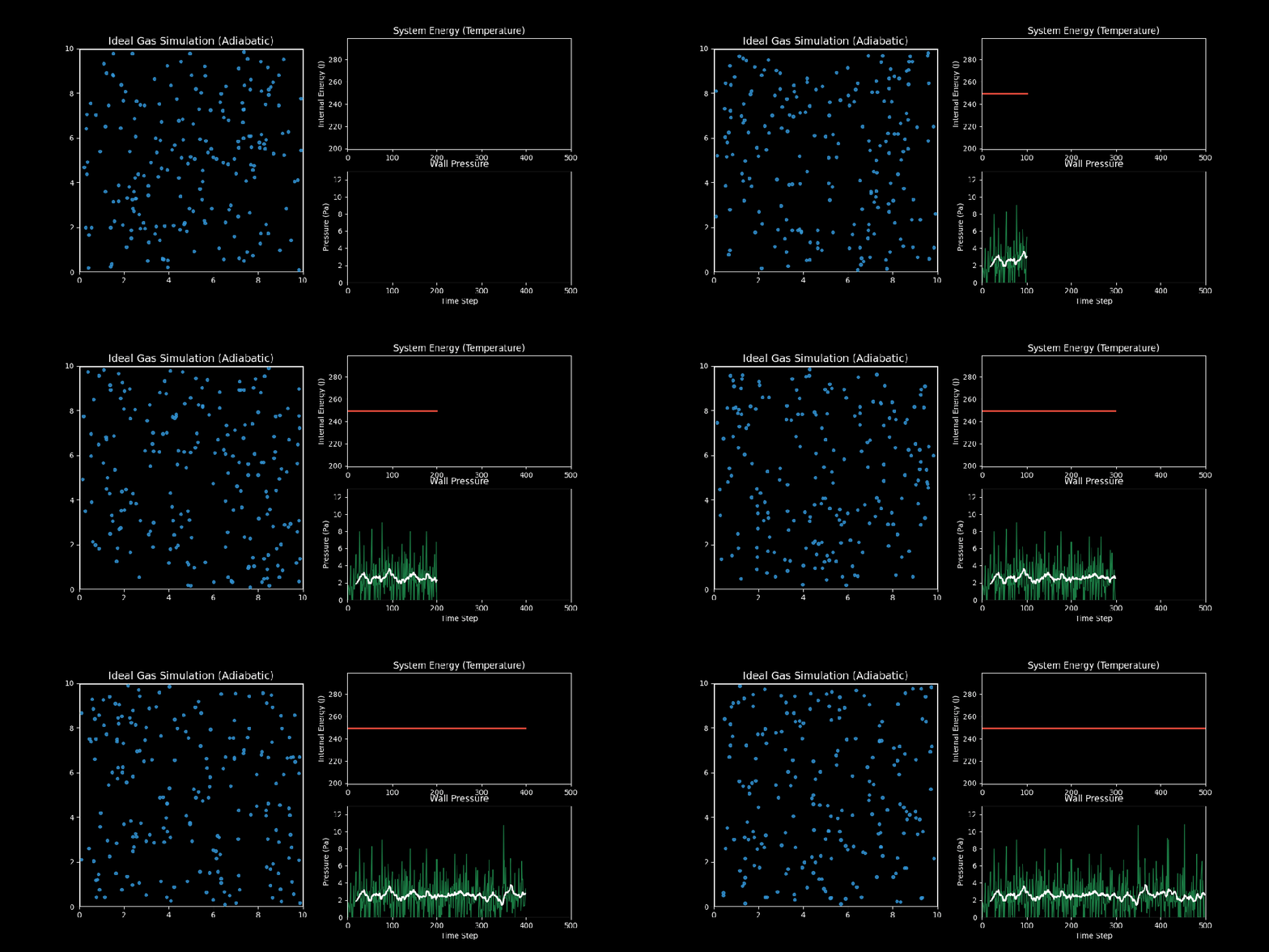
• 左图（分子运动）：你可以看到蓝色的气体分子在容器内做无规则的热运动（布朗运动），并不断撞击墙壁。
• 右上图（内能/温度）：红线显示了系统的总动能。你会发现它是一条完美的水平直线。这验证了能量守恒定律——在没有外力做功和热交换的情况下，理想气体的内能是恒定的。
• 右下图（压力）：绿线是瞬时压力，白线是移动平均压力。虽然每个瞬间的撞击力度是随机波动的（噪声），但从统计平均来看，压力稳定在一个恒定的数值。这就解释了为什么宏观上我们能测量到稳定的气压。

绝热压缩与膨胀：活塞模型

在前面的模拟中，容器体积是固定的。现在，让我们引入一个可移动的活塞（Piston），通过改变容器体积来对气体做功。

1. 物理过程

• 压缩过程（Compression）：活塞向内移动，分子撞击活塞时会被反弹回来，且速度增加（类似于你用网球拍击球，球速会变快）。外界对气体做功，气体内能增加，温度升高。
• 膨胀过程（Expansion）：活塞向外移动，分子撞击活塞时反弹速度减小（类似于球打在后退的球拍上）。气体对外界做功，内能减少，温度降低。

2. 代码实现

我们需要修改碰撞检测逻辑，处理动墙（Moving Wall）碰撞：

其中  是活塞速度。

完整代码如下：

import numpy as npimport matplotlib.pyplot as pltfrom matplotlib.animation import FuncAnimation# 理想气体绝热压缩/膨胀模拟# 1. 系统参数N = 100# 分子数量BOX_WIDTH_INIT = 10.0BOX_HEIGHT = 10.0V_MAX = 2.0# 初始速度MASS = 1.0RADIUS = 0.1DT = 0.05STEPS = 600# 活塞运动参数PISTON_SPEED = 0.02# 活塞速度 (正值压缩，负值膨胀)# 我们设计一个周期运动：压缩 -> 膨胀defget_piston_pos(step):# 简单的正弦运动模拟活塞# 周期 600 步    phase = step / STEPS * 2 * np.pi# 宽度在 5.0 到 10.0 之间变化return7.5 + 2.5 * np.cos(phase)defget_piston_vel(step):# 位置的导数    phase = step / STEPS * 2 * np.pireturn-2.5 * np.sin(phase) * (2 * np.pi / STEPS / DT)# 2. 初始化状态pos = np.random.uniform(RADIUS, BOX_WIDTH_INIT - RADIUS, size=(N, 2))pos[:, 1] = np.random.uniform(RADIUS, BOX_HEIGHT - RADIUS, size=N) # y 轴范围固定vel = np.random.uniform(-V_MAX, V_MAX, size=(N, 2))# 存储历史history = {'pos': [], 'ke': [], 'pressure': [], 'volume': [], 'box_width': []}# 3. 模拟循环for step_idx in range(STEPS):# 当前容器宽度 (由活塞位置决定)    current_width = get_piston_pos(step_idx)    next_width = get_piston_pos(step_idx + 1)# 活塞瞬时速度    v_piston = (next_width - current_width) / DT    # 更新分子位置    pos += vel * DT    # 碰撞检测    impulse = 0.0# --- 右侧活塞墙壁 (动墙) ---# 只有 x > current_width - RADIUS 的分子可能碰撞    mask_piston = pos[:, 0] > current_width - RADIUS    if np.any(mask_piston):# 修正位置        pos[mask_piston, 0] = current_width - RADIUS        # 弹性碰撞公式 (动墙)# v_new = 2 * v_wall - v_old# 这里 v_wall = v_piston        v_old_x = vel[mask_piston, 0]        v_new_x = 2 * v_piston - v_old_x        vel[mask_piston, 0] = v_new_x        # 动量变化 (相对于静止参考系)# 但计算压力时通常用相对动量变化，或者直接用 F = ma# 这里简化：压力来自于分子对活塞的冲量# 冲量 I = m * (v_new - v_old)        impulse += np.sum(MASS * np.abs(v_new_x - v_old_x))        # --- 左侧、上侧、下侧 (静墙) ---    mask_left = pos[:, 0] < RADIUSif np.any(mask_left):        pos[mask_left, 0] = RADIUS        vel[mask_left, 0] *= -1    mask_bottom = pos[:, 1] < RADIUSif np.any(mask_bottom):        pos[mask_bottom, 1] = RADIUS        vel[mask_bottom, 1] *= -1    mask_top = pos[:, 1] > BOX_HEIGHT - RADIUSif np.any(mask_top):        pos[mask_top, 1] = BOX_HEIGHT - RADIUS        vel[mask_top, 1] *= -1# 记录数据    ke = 0.5 * MASS * np.sum(vel**2)    pressure = impulse / DT / BOX_HEIGHT # 只计算活塞受到的压力 P=F/L        history['pos'].append(pos.copy())    history['ke'].append(ke)    history['pressure'].append(pressure)    history['box_width'].append(current_width)    history['volume'].append(current_width * BOX_HEIGHT)# 动态可视化plt.style.use('dark_background')fig = plt.figure(figsize=(10, 10))# 调整布局，增加 hspace 防止重叠gs = fig.add_gridspec(3, 1, height_ratios=[2, 1, 1], hspace=0.4)# --- 上图：活塞运动 ---ax_box = fig.add_subplot(gs[0])ax_box.set_xlim(0, 12)ax_box.set_ylim(0, 10)ax_box.set_aspect('equal')ax_box.set_title("Adiabatic Compression/Expansion", color='white', fontsize=14)ax_box.set_xlabel("Volume Change (Piston Movement)")# 容器边界wall_top = ax_box.axhline(BOX_HEIGHT, color='white', lw=2)wall_bottom = ax_box.axhline(0, color='white', lw=2)wall_left = ax_box.axvline(0, color='white', lw=2)# 活塞piston_line = ax_box.axvline(BOX_WIDTH_INIT, color='#e74c3c', lw=4, label='Piston')# 分子particles, = ax_box.plot([], [], 'o', color='#3498db', markersize=5, alpha=0.8)# --- 中图：温度 (动能) ---ax_temp = fig.add_subplot(gs[1])ax_temp.set_xlim(0, STEPS)ax_temp.set_ylim(np.min(history['ke'])*0.8, np.max(history['ke'])*1.2)ax_temp.set_ylabel("Internal Energy (Temp)")ax_temp.grid(True, linestyle='--', alpha=0.3)line_ke, = ax_temp.plot([], [], '-', color='#f1c40f', lw=2)# --- 下图：压力 ---ax_press = fig.add_subplot(gs[2])ax_press.set_xlim(0, STEPS)ax_press.set_ylim(0, np.max(history['pressure'])*1.5)ax_press.set_ylabel("Pressure on Piston")ax_press.set_xlabel("Time Step")ax_press.grid(True, linestyle='--', alpha=0.3)line_press, = ax_press.plot([], [], '-', color='#2ecc71', lw=1, alpha=0.5)line_press_avg, = ax_press.plot([], [], '-', color='white', lw=2)defupdate(frame):# 降采样：每 3 步取 1 帧# 总步数 600 / 3 = 200 帧 < 300    skip = 3    idx = frame * skipif idx >= STEPS: idx = STEPS - 1# 1. 更新活塞和分子    width = history['box_width'][idx]    piston_line.set_xdata([width, width])        p = history['pos'][idx]    particles.set_data(p[:, 0], p[:, 1])    # 2. 更新曲线# xdata 对应模拟步数，而不是帧数    current_step = idx    xdata = range(current_step + 1)        line_ke.set_data(xdata, history['ke'][:current_step+1])        press_data = history['pressure'][:current_step+1]    line_press.set_data(xdata, press_data)    if current_step > 10:        avg_p = np.convolve(press_data, np.ones(10)/10, mode='valid')        line_press_avg.set_data(range(9, current_step+1), avg_p)        return piston_line, particles, line_ke, line_press, line_press_avgframes = STEPS // 3ani = FuncAnimation(fig, update, frames=frames, interval=30, blit=True)ani.save('../images/05_piston_simulation.gif', writer='pillow', fps=20)print("Piston animation saved to ../images/05_piston_simulation.gif")

3. 可视化结果

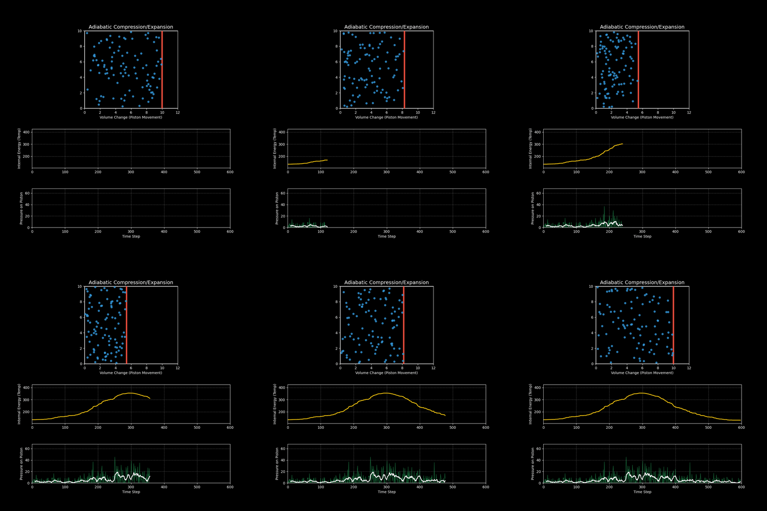
• 上图：展示了活塞（红线）的周期性运动。你可以看到当活塞向左压缩时，分子运动明显变剧烈；当活塞向右膨胀时，分子运动变缓慢。
• 中图（温度/内能）：黄线显示了系统的温度变化。压缩升温，膨胀降温，这正是柴油发动机点火（压缩引燃）和冰箱制冷（膨胀吸热）的基本原理。
• 下图（压力）：绿线显示了气体对活塞的压力。体积越小，压力越大（波义耳定律），且温度升高进一步加剧了压力的上升。

总结

通过这个模拟，我们成功地架起了微观粒子运动与宏观热力学定律之间的桥梁：

1. 微观随机性（分子的混乱运动）导致了宏观稳定性（稳定的压力和温度）。
2. 能量守恒在微观碰撞中得到了严格的体现。
3. 压力本质上是大量分子撞击效应的统计平均。

这种分子动力学模拟方法不仅可以用于理想气体，通过引入分子间作用力等等，还可以模拟液体、固体甚至相变过程。