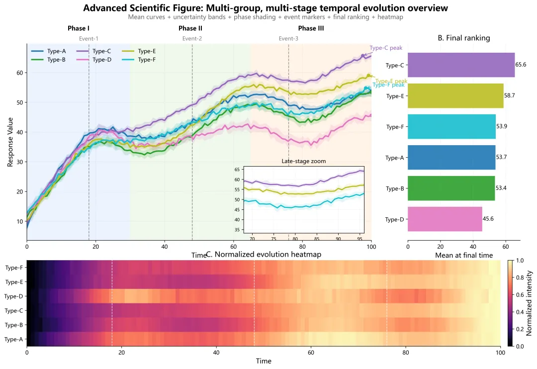
import numpy as npimport pandas as pdimport matplotlib.pyplot as pltfrom matplotlib.gridspec import GridSpecfrom matplotlib import font_managerfrom mpl_toolkits.axes_grid1.inset_locator import inset_axesfrom pathlib import Path# 0. 基础设置def set_chinese_font(): """自动寻找常见中文字体,避免中文乱码。""" candidates = [ "Microsoft YaHei", "SimHei", "Noto Sans CJK SC", "Source Han Sans CN", "WenQuanYi Zen Hei", "Arial Unicode MS" ] available = {f.name for f in font_manager.fontManager.ttflist} for font_name in candidates: if font_name in available: plt.rcParams["font.sans-serif"] = [font_name] break plt.rcParams["axes.unicode_minus"] = Falseset_chinese_font()plt.rcParams["figure.dpi"] = 160plt.rcParams["savefig.dpi"] = 300plt.rcParams["font.size"] = 11plt.rcParams["axes.labelsize"] = 12plt.rcParams["axes.titlesize"] = 13plt.rcParams["legend.fontsize"] = 10plt.rcParams["xtick.labelsize"] = 10plt.rcParams["ytick.labelsize"] = 10OUTDIR = Path("python_advanced_figure_output")OUTDIR.mkdir(parents=True, exist_ok=True)np.random.seed(42)# 1. 生成模拟数据time = np.linspace(0, 100, 121)groups = ["Type-A", "Type-B", "Type-C", "Type-D", "Type-E", "Type-F"]n_rep = 10params = { "Type-A": dict(base=8, amp=34, tau=16, s1=7, s2=10, drop=4, osc=1.8, drift=2.0, phase=0.2, noise=1.2), "Type-B": dict(base=10, amp=28, tau=22, s1=10, s2=14, drop=7, osc=1.5, drift=1.0, phase=1.0, noise=1.4), "Type-C": dict(base=7, amp=37, tau=14, s1=5, s2=18, drop=5, osc=2.0, drift=1.8, phase=1.8, noise=1.0), "Type-D": dict(base=12, amp=25, tau=18, s1=12, s2=8, drop=9, osc=1.2, drift=0.8, phase=2.4, noise=1.6), "Type-E": dict(base=9, amp=31, tau=20, s1=8, s2=16, drop=3, osc=1.7, drift=2.5, phase=0.6, noise=1.3), "Type-F": dict(base=11, amp=29, tau=17, s1=6, s2=12, drop=6, osc=1.4, drift=1.5, phase=2.0, noise=1.5),}records = []for g in groups: p = params[g] for rep in range(1, n_rep + 1): base_curve = p["base"] + p["amp"] * (1 - np.exp(-time / p["tau"])) pulse_1 = p["s1"] * np.exp(-((time - 20) ** 2) / (2 * 7 ** 2)) pulse_2 = p["s2"] / (1 + np.exp(-(time - 55) / 5)) pulse_3 = -p["drop"] * np.exp(-((time - 82) ** 2) / (2 * 8 ** 2)) osc = p["osc"] * np.sin(time / 8 + p["phase"]) drift = p["drift"] * (time / 100) rep_scale = np.clip(np.random.normal(1.0, 0.15), 0.7, 1.3) noise = np.random.normal(0, p["noise"] * rep_scale, size=time.size) value = base_curve + pulse_1 + pulse_2 + pulse_3 + osc + drift + noise value = np.clip(value, 0, None) for t, y in zip(time, value): records.append([g, rep, t, y])df_raw = pd.DataFrame(records, columns=["group", "replicate", "time", "value"])csv_path = OUTDIR / "synthetic_multigroup_time_series.csv"df_raw.to_csv(csv_path, index=False, encoding="utf-8-sig")df_stat = ( df_raw.groupby(["group", "time"])["value"] .agg(mean="mean", std="std") .reset_index())# 2. 绘图参数colors = plt.cm.tab10(np.linspace(0, 1, len(groups)))phase_spans = [ (0, 30, "Phase I", "#EAF2FF"), (30, 65, "Phase II", "#EEF8EA"), (65, 100, "Phase III", "#FFF3E6"),]events = [ (18, "Event-1"), (48, "Event-2"), (76, "Event-3"),]# 3. 构建图版fig = plt.figure(figsize=(16, 10))gs = GridSpec( nrows=2, ncols=2, width_ratios=[4.6, 1.5], height_ratios=[3.2, 1.4], wspace=0.16, hspace=0.14)ax_main = fig.add_subplot(gs[0, 0])ax_rank = fig.add_subplot(gs[0, 1])ax_heat = fig.add_subplot(gs[1, :])# 给顶部多留一点空间fig.subplots_adjust(top=0.87)# 3.1 主图背景阶段色块for x0, x1, label, facecolor in phase_spans: ax_main.axvspan(x0, x1, color=facecolor, alpha=0.9, zorder=0) ax_main.text( (x0 + x1) / 2, 1.06, label, # 往上移 transform=ax_main.get_xaxis_transform(), ha="center", va="bottom", fontsize=11, fontweight="bold" )# 关键事件线for x, label in events: ax_main.axvline(x, color="gray", linestyle="--", linewidth=1.2, alpha=0.8, zorder=1) ax_main.text( x, 1.01, label, transform=ax_main.get_xaxis_transform(), ha="center", va="bottom", color="gray", fontsize=10 )# 3.2 主图:均值曲线 + 误差带 + 峰值标注peak_infos = []for i, g in enumerate(groups): sub = df_stat[df_stat["group"] == g].copy() x = sub["time"].to_numpy() y = sub["mean"].to_numpy() s = sub["std"].to_numpy() ax_main.fill_between( x, y - s, y + s, color=colors[i], alpha=0.16, linewidth=0 ) ax_main.plot( x, y, color=colors[i], linewidth=2.5, label=g ) idx_peak = np.argmax(y) px, py = x[idx_peak], y[idx_peak] ax_main.scatter(px, py, s=28, color=colors[i], zorder=5) peak_infos.append((g, px, py, colors[i]))ax_main.set_xlim(0, 100)ax_main.set_xlabel("Time")ax_main.set_ylabel("Response Value")ax_main.grid(alpha=0.18, linestyle="--")ax_main.legend(ncol=3, frameon=False, loc="upper left")ax_main.spines["top"].set_visible(False)ax_main.spines["right"].set_visible(False)top3_peak = sorted(peak_infos, key=lambda k: k[2], reverse=True)[:3]offsets = [(2, 2.5), (2, -2.0), (2, 1.0)]for (g, px, py, c), (dx, dy) in zip(top3_peak, offsets): ax_main.annotate( f"{g} peak", xy=(px, py), xytext=(px + dx, py + dy), fontsize=10, color=c, arrowprops=dict(arrowstyle="->", lw=1.0, color=c), ha="left", va="center" )# 3.3 主图内嵌放大图last_time = df_stat["time"].max()df_last = df_stat[df_stat["time"] == last_time].copy()top3_groups = df_last.sort_values("mean", ascending=False)["group"].head(3).tolist()ax_inset = inset_axes(ax_main, width="35%", height="34%", loc="lower right", borderpad=1.3)for i, g in enumerate(groups): if g not in top3_groups: continue sub = df_stat[df_stat["group"] == g].copy() x = sub["time"].to_numpy() y = sub["mean"].to_numpy() s = sub["std"].to_numpy() c = colors[groups.index(g)] ax_inset.fill_between(x, y - s, y + s, color=c, alpha=0.12, linewidth=0) ax_inset.plot(x, y, color=c, linewidth=2)ax_inset.set_xlim(68, 96)late_mask = df_stat["time"].between(68, 96)ymin = (df_stat.loc[late_mask, "mean"] - df_stat.loc[late_mask, "std"]).min() - 1ymax = (df_stat.loc[late_mask, "mean"] + df_stat.loc[late_mask, "std"]).max() + 1ax_inset.set_ylim(ymin, ymax)ax_inset.set_title("Late-stage zoom", fontsize=10)ax_inset.grid(alpha=0.15, linestyle="--")ax_inset.tick_params(labelsize=8)# 3.4 右侧:末期均值排名rank_df = df_last.sort_values("mean", ascending=True).reset_index(drop=True)bar_colors = [colors[groups.index(g)] for g in rank_df["group"]]ax_rank.barh(rank_df["group"], rank_df["mean"], color=bar_colors, alpha=0.9)for y_pos, val in enumerate(rank_df["mean"]): ax_rank.text(val + 0.3, y_pos, f"{val:.1f}", va="center", fontsize=10)ax_rank.set_title("B. Final ranking")ax_rank.set_xlabel("Mean at final time")ax_rank.grid(axis="x", alpha=0.18, linestyle="--")ax_rank.spines["top"].set_visible(False)ax_rank.spines["right"].set_visible(False)ax_rank.spines["left"].set_visible(False)# 3.5 底部:归一化热图heat = ( df_stat.pivot(index="group", columns="time", values="mean") .reindex(groups))heat_norm = heat.copy()row_min = heat.min(axis=1)row_max = heat.max(axis=1)den = (row_max - row_min).replace(0, 1)for g in groups: heat_norm.loc[g] = (heat.loc[g] - row_min[g]) / den[g]im = ax_heat.imshow( heat_norm.to_numpy(), aspect="auto", origin="lower", cmap="magma", extent=[time.min(), time.max(), -0.5, len(groups) - 0.5])ax_heat.set_yticks(range(len(groups)))ax_heat.set_yticklabels(groups)ax_heat.set_xlabel("Time")ax_heat.set_title("C. Normalized evolution heatmap")for x, _ in events: ax_heat.axvline(x, color="white", linestyle="--", linewidth=1.0, alpha=0.85)cbar = fig.colorbar(im, ax=ax_heat, fraction=0.025, pad=0.015)cbar.set_label("Normalized intensity")ax_heat.spines["top"].set_visible(False)ax_heat.spines["right"].set_visible(False)# 4. 总标题与导出fig.suptitle( "Advanced Scientific Figure: Multi-group, multi-stage temporal evolution overview", fontsize=16, fontweight="bold", y=0.97)# 往下移一点fig.text( 0.5, 0.932, "Mean curves + uncertainty bands + phase shading + event markers + final ranking + heatmap", ha="center", fontsize=11, color="dimgray")png_path = OUTDIR / "advanced_multigroup_temporal_overview_fixed2.png"svg_path = OUTDIR / "advanced_multigroup_temporal_overview_fixed2.svg"fig.savefig(png_path, bbox_inches="tight")fig.savefig(svg_path, bbox_inches="tight")plt.show()print("模拟数据已保存:", csv_path)print("PNG图片已保存:", png_path)print("SVG图片已保存:", svg_path)

 10个月宝宝每天需要喝多少奶粉?