在上一节中,我们观察到:
但一个根本问题仍然存在:
模型误差究竟来自哪里?
1问题设定
设真实模型:
我们用模型 进行拟合。
👉 目标:
分析预测误差:
2分解推导
展开:
代入:
展开平方:
由于:
👉 得:
继续分解第一项:
引入期望:
3最终结果
4三个部分解释
1️⃣ Bias(偏差)
👉 含义:
模型“平均预测”与真实函数的差距
2️⃣ Variance(方差)
👉 含义:
模型对数据扰动的敏感性
3️⃣ Noise(不可约误差)
👉 含义:
数据本身的随机性(无法消除)
5直觉理解(非常关键)
👉 核心矛盾:
无法同时最小化 Bias 和 Variance
6Python验证(核心实验)
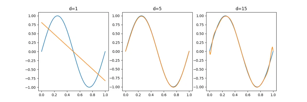
# file: bias_variance_simulation.pyimport numpy as npimport matplotlib.pyplot as pltdeftrue_function(x):return np.sin(2*np.pi*x)deffit_model(x, y, degree):return np.polyfit(x, y, degree)defpredict(coeffs, x):return np.polyval(coeffs, x)defmain(): np.random.seed(0) x_test = np.linspace(0,1,100) y_true = true_function(x_test) degrees = [1, 5, 15] plt.figure(figsize=(12,4))for i, d in enumerate(degrees): preds = []for _ in range(100): x_train = np.linspace(0,1,20) y_train = true_function(x_train) + np.random.normal(0,0.2,20) coeffs = fit_model(x_train, y_train, d) y_pred = predict(coeffs, x_test) preds.append(y_pred) preds = np.array(preds) mean_pred = np.mean(preds, axis=0) bias = np.mean((mean_pred - y_true)**2) variance = np.mean(np.var(preds, axis=0)) print(f"degree={d}, bias={bias:.4f}, var={variance:.4f}") plt.subplot(1,3,i+1) plt.plot(x_test, y_true, label="true") plt.plot(x_test, mean_pred, label="mean pred") plt.title(f"d={d}") plt.show()if __name__ == "__main__": main()
执行结果如下:7结果解释
你会看到:
👉 直接验证理论
8正则化的作用
Ridge / Lasso:
👉 作用:
👉 结论:
正则化 = 在 Bias 和 Variance 之间做权衡
9Python验证(正则化效果)
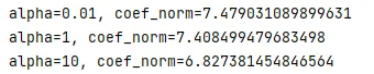
# file: ridge_bias_variance.pyimport numpy as npfrom sklearn.linear_model import Ridgedefmain(): np.random.seed(0) X = np.random.randn(100,10) beta_true = np.array([1,2,3,4,5,0,0,0,0,0]) y = X @ beta_true + np.random.randn(100)for alpha in [0.01, 1, 10]: model = Ridge(alpha=alpha) model.fit(X,y) print(f"alpha={alpha}, coef_norm={np.linalg.norm(model.coef_)}")if __name__ == "__main__": main()
执行结果如下: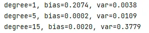
 10个月宝宝每天需要喝多少奶粉?
