编者按
虽然说最新版的spaceranger v4支持直接导出细胞分割后的结果,但我们还是提供一个从图像中手动进行细胞分割的方案Cellpose和CellSAM,希望有所帮助。
steorra
Space Ranger v4.0 为 Visium HD Spatial Gene Expression 和 Visium HD 3' Spatial Gene Expression 引入了细胞核与细胞级分割结果。
而在这之前,社区里也已经出现了多种适用于高分辨率图像的细胞分割方案,例如 StarDist 和 Cellpose。原始的 bin2cell 工作流集成的是 StarDist;但是它要安装tensorflow,这有点破坏我们的torhc环境,这里我们保留 bin2cell 的整体思路,但把分割环节改写为基于 Python 的 Cellpose和CellSAM 后端,这样整条流程可以保持在纯 Python的torch 环境中完成。
本教程将演示如何在 OmicVerse 中把 Visium HD 的 2 µm bin、H&E 图像、Cellpose 分割以及 bin-to-cell 聚合串成一条完整流程。主线很明确:从超高分辨率 bin 出发,尽可能恢复接近真实细胞形状的对象,并把结果整理成可直接用于下游空间分析的细胞级数据。
import omicverse as ov
import scanpy as sc
ov.plot_set(font_path='Arial')

# 启用自动重载,便于开发时即时同步代码修改
%load_ext autoreload
%autoreload 2
🔬 Starting plot initialization...
Using already downloaded Arial font from: /tmp/omicverse_arial.ttf
Registered as: Arial
🧬 Detecting GPU devices…
✅ NVIDIA CUDA GPUs detected: 1
    • [CUDA 0] NVIDIA H100 80GB HBM3
      Memory: 79.1 GB | Compute: 9.0

   ____            _     _    __
  / __ \____ ___  (_)___| |  / /__  _____________
 / / / / __ `__ \/ / ___/ | / / _ \/ ___/ ___/ _ \
/ /_/ / / / / / / / /__ | |/ /  __/ /  (__  )  __/
\____/_/ /_/ /_/_/\___/ |___/\___/_/  /____/\___/

🔖 Version: 2.1.2rc1   📚 Tutorials: https://omicverse.readthedocs.io/
✅ plot_set complete.
加载数据集
Visium HD 很可能会成为液滴式单细胞测序之后最重要的一类空间技术之一。由于它在 2 µm bin 上记录表达信号,这份数据已经非常接近亚细胞分辨率。于是分析上会出现一个很现实的问题:我们是否可以不急着把这些 bin 粗略合并成更大的 pseudo-spot,而是借助图像和分割结果,更准确地重建细胞级对象?
Bin2cell 正是围绕这个问题设计的。它首先校正由 bin 尺寸变化引入的技术效应,然后基于图像分割把 bin 分配给候选细胞,最终得到一个可直接进入下游分析的细胞级 AnnData 对象。在这个 notebook 中,我们同时使用形态学图像和由基因表达构造出的图像表示,因为这两种输入各自覆盖了不同的分割失败场景。
这里使用的计数矩阵和 H&E 图像下载自 https://www.10xgenomics.com/datasets/visium-hd-cytassist-gene-expression-libraries-of-human-crc。
from pathlib import Path

defprint_tree(path: Path, prefix: str = ""):
    print(prefix + path.name + "/")
for child in path.iterdir():
if child.is_dir():
            print_tree(child, prefix + "    ")
else:
            print(prefix + "    " + child.name)

print_tree(Path("binned_outputs/square_002um/"))
square_002um/
    spatial/
        aligned_fiducials.jpg
        detected_tissue_image.jpg
        tissue_positions.parquet
        aligned_tissue_image.jpg
        tissue_lowres_image.png
        cytassist_image.tiff
        tissue_hires_image.png
        scalefactors_json.json
    raw_feature_bc_matrix.h5
    filtered_feature_bc_matrix/
        barcodes.tsv.gz
        features.tsv.gz
        matrix.mtx.gz
    raw_probe_bc_matrix.h5
    filtered_feature_bc_matrix.h5
    raw_feature_bc_matrix/
        barcodes.tsv.gz
        features.tsv.gz
        matrix.mtx.gz
path = "binned_outputs/square_002um/"
source_image_path = "Visium_HD_Human_Colon_Cancer_tissue_image.btf"
# os.chdir('./')

# 为 Cellpose 中间文件创建输出目录
import os
os.makedirs("stardist", exist_ok=True)
当前加载计数矩阵仍然需要一个定制的读取函数,因为 10x 已将 spot/bin 坐标移入 Parquet 文件,并把组织图像单独存放在spatial/目录下。binned 目录里通常只保留这些图像的符号链接,数据跨机器复制时这些链接可能会失效。
adata = ov.space.read_visium_10x(path, source_image_path=source_image_path)
adata.var_names_make_unique()
adata
AnnData object with n_obs × n_vars = 8731400 × 18085
    obs: 'in_tissue', 'array_row', 'array_col'
    var: 'gene_ids', 'feature_types', 'genome'
    uns: 'spatial'
    obsm: 'spatial'
在进入分割之前,先做一个轻量过滤:要求基因至少出现在 3 个 bin 中,并要求每个 bin 至少包含一些计数信息。由于 2 µm 分辨率下矩阵仍然非常稀疏,这一步主要用于去掉明显的空 bin,而不会改变整体生物学结构。
ov.pp.filter_genes(adata, min_cells=3)
ov.pp.filter_cells(adata, min_counts=1)
adata
🔍 Filtering genes...
   Parameters: min_cells≥3
✓ Filtered: 27 genes removed

╭─ SUMMARY: filter_genes ────────────────────────────────────────────╮
│  Duration: 9.769s                                                  │
│  Shape:    8,731,400 x 18,085 -> 8,731,400 x 18,058                │
│                                                                    │
│  CHANGES DETECTED                                                  │
│  ────────────────                                                  │
╰────────────────────────────────────────────────────────────────────╯
🔍 Filtering cells...
   Parameters: min_counts≥1
✓ Filtered: 475,557 cells removed

╭─ SUMMARY: filter_cells ────────────────────────────────────────────╮
│  Duration: 10.7018s                                                │
│  Shape:    8,731,400 x 18,058 -> 8,255,843 x 18,058                │
│                                                                    │
│  CHANGES DETECTED                                                  │
│  ────────────────                                                  │
╰────────────────────────────────────────────────────────────────────╯
AnnData object with n_obs × n_vars = 8255843 × 18058
    obs: 'in_tissue', 'array_row', 'array_col'
    var: 'gene_ids', 'feature_types', 'genome'
    uns: 'spatial', 'history_log'
    obsm: 'spatial'
使用 Cellpose 对 H&E 图像进行细胞分割
在这条流程里,bin2cell 会同时对 H&E 图像和一个基于基因表达构造出的图像表示做分割。输入图像的分辨率由mpp参数控制,即 microns per pixel(每个像素对应多少微米)。例如,如果直接把原始阵列坐标(.obs['array_row']和.obs['array_col'])当作图像网格,那么每个像素就对应 2 µm,因此这种表示的mpp=2。
在本地测试中,这个结肠样本使用0.3到0.5左右的mpp都能取得不错效果。这里选择mpp=0.3,因为它能在 H&E 图像上保留更清晰的形态细节,有利于 Cellpose 做边界判断。
ov.space.visium_10x_hd_cellpose_he(
    adata,
    mpp=0.3,
    he_save_path="stardist/he_colon1.tiff",
    prob_thresh=0,
    flow_threshold=0.4,
    gpu=True,
    buffer=150,
    backend='tifffile',
)
he_save_path stardist/he_colon1.tiff already exists, skipping image generation
Cropped spatial coordinates key: spatial_cropped_150_buffer
Image key: 0.3_mpp_150_buffer
no seeds found in get_masks_torch - no masks found.
初始的 H&E 分割更像是提供以细胞核为中心的种子,而完整细胞通常会明显超出细胞核范围。因此,ov.space.visium_10x_hd_cellpose_expand()会把每个已标记对象向周围 bin 扩展。
使用max_bin_distance时,距离某个标记种子不超过固定步数的 bin 会被划入同一个细胞。另一种方式是设置algorithm='volume_ratio':它会根据种子对象的大小,为每个标签估计一个单独的扩展距离,这个估计基于核体积与细胞体积近似线性相关的假设,比例由volume_ratio(默认4)控制。如果某个 bin 与多个细胞核的距离完全相同,则会借助 PCA 空间中的表达相似性来打破平局。
ov.space.visium_10x_hd_cellpose_expand(
    adata,
    labels_key='labels_he',
    expanded_labels_key="labels_he_expanded",
    max_bin_distance=4,
)
使用 Cellpose 对 GEX 图像进行细胞分割
H&E 分割并不保证完美。有些区域虽然有明显表达信号,却缺少可见的细胞核作为种子;另一些区域里的细胞核形态异常,也可能被图像模型漏掉。此时,对每个 bin 的总表达量构造图像并再次做分割,往往能补回一部分漏检对象。
不过,基于表达量的分割在稀疏组织中效果最好;如果组织过于致密,相邻细胞的信号容易混在一起,边界会变得难以区分。因此,这里把它作为次级的目标识别来源,只在 H&E 难以覆盖的地方补充对象。
这里的输入图像是每个 bin 总计数的平滑表示,先施加sigma=5像素的高斯滤波。随后继续使用 Cellpose 来识别更接近“整细胞”的对象,而不是仅识别细胞核,因此这一步之后不需要再额外做标签扩展。和 H&E 分割一样,调低prob_thresh会让判定更宽松;调高nms_thresh则要求候选对象之间有更强重叠才会被合并,在较致密区域有时会更稳。
ov.space.visium_10x_hd_cellpose_gex(
    adata,
    obs_key="n_counts_adjusted",
    log1p=False,
    mpp=0.3,
    sigma=5,
    gex_save_path="stardist/gex_colon1.tiff",
    prob_thresh=0.01,
    nms_thresh=0.1,
    gpu=True,
    buffer=150,
)
gex_save_path stardist/gex_colon1.tiff already exists, skipping grid_image
ov.space.salvage_secondary_labels(
    adata,
    primary_label="labels_he_expanded",
    secondary_label="labels_gex",
    labels_key="labels_joint"
)
Salvaged 864 secondary labels
adata.write('visium_hd/adata_cellpose.h5ad')
Bin to Cell
到这里为止,bin 已经完成去条纹校正,并且分别基于 H&E 和 GEX 分割被分配给候选细胞。接下来就可以把 bin 级计数真正聚合成细胞级表达谱。
cdata = ov.space.bin2cell(
    adata, labels_key="labels_joint",
    spatial_keys=["spatial", "spatial_cropped_150_buffer"])
cdata
AnnData object with n_obs × n_vars = 84853 × 18058
    obs: 'object_id', 'bin_count', 'array_row', 'array_col', 'labels_joint_source', 'geometry', 'cellid'
    var: 'gene_ids', 'feature_types', 'genome'
    uns: 'spatial', 'omicverse_io'
    obsm: 'spatial', 'spatial_cropped_150_buffer'
ov.pl.embedding(
    cdata,
    basis='spatial_cropped_150_buffer',
    color=['COL1A1'],
    vmax='p99.2',cmap='RdBu_r',
    size=5,
)
<Figure size 320x320 with 2 Axes>
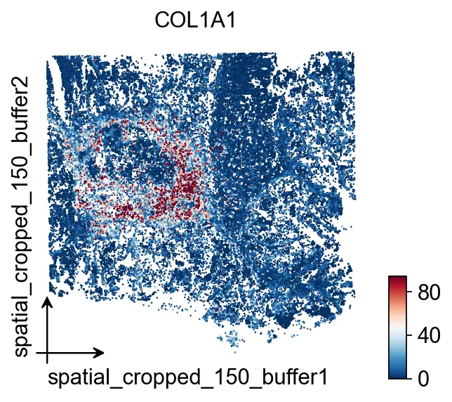 细胞级对象构建完成后,先用
COL1A1检查整体空间表达布局。可视化
# 定义一个掩码,后续可以方便地重复抽取这块局部区域
mask = ((adata.obs['array_row'] >= 2225) &
        (adata.obs['array_row'] <= 2275) &
        (adata.obs['array_col'] >= 1400) &
        (adata.obs['array_col'] <= 1450))
print(f'Subregion: {mask.sum()} bins')
Subregion: 2601 bins
bdata = adata[mask]
# 0 表示未分配给任何细胞
bdata = bdata[bdata.obs['labels_he']>0]
bdata.obs['labels_he'] = bdata.obs['labels_he'].astype(str)

sc.pl.spatial(bdata, color=[None, "labels_he"], img_key="0.3_mpp_150_buffer",
              basis="spatial_cropped_150_buffer")
<Figure size 772.8x320 with 2 Axes>
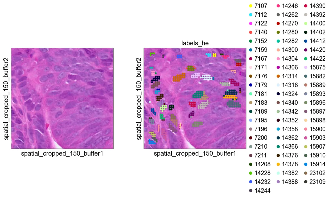 这张局部图展示的是 H&E 分割得到的原始种子标签。
bdata = adata[mask]
# 0 表示未分配给任何细胞
bdata = bdata[bdata.obs['labels_he_expanded']>0]
bdata.obs['labels_he_expanded'] = bdata.obs['labels_he_expanded'].astype(str)

sc.pl.spatial(bdata, color=[None, "labels_he_expanded"], img_key="0.3_mpp_150_buffer",
              basis="spatial_cropped_150_buffer")
<Figure size 772.8x320 with 2 Axes>
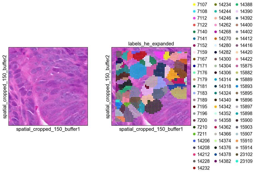 扩展后的 H&E 标签更接近完整细胞范围。
bdata = adata[mask]
# 0 表示未分配给任何细胞
bdata = bdata[bdata.obs['labels_gex']>0]
bdata.obs['labels_gex'] = bdata.obs['labels_gex'].astype(str)

sc.pl.spatial(bdata, color=[None, "labels_gex"], img_key="0.3_mpp_150_buffer",
              basis="spatial_cropped_150_buffer")
<Figure size 772.8x320 with 3 Axes>
 GEX 分割结果可以补充 H&E 难以覆盖的对象。
bdata = adata[mask]

# 0 表示未分配给任何细胞
bdata = bdata[bdata.obs['labels_joint']>0]
bdata.obs['labels_joint'] = bdata.obs['labels_joint'].astype(str)

sc.pl.spatial(bdata, color=[None, "labels_joint_source",
"labels_joint"], img_key="0.3_mpp_150_buffer",
              basis="spatial_cropped_150_buffer")
<Figure size 1159.2x320 with 3 Axes>
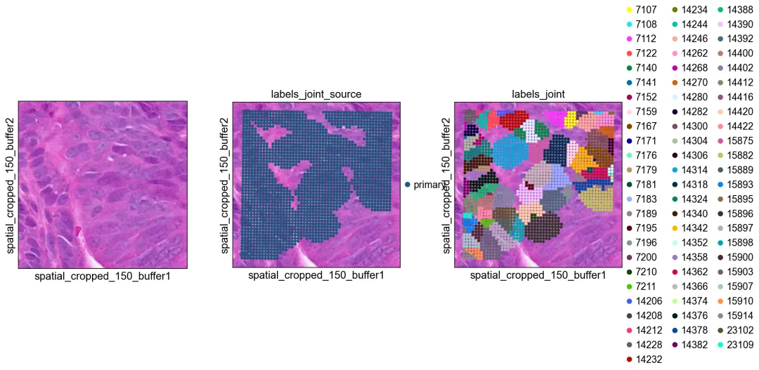 联合标签把 H&E 与 GEX 两路结果整合到同一个对象空间中。
导出为 SpaceRanger v4 格式
ov.space.write_visium_hd_cellseg()可以把细胞级 AnnData 导出成与 SpaceRanger v4 分割输出一致的目录结构。这样一来,Cellpose 得到的分割结果就具备了更好的可移植性:任何已经支持 SpaceRanger v4 cell-segmentation 输出的工具,都可以重新读回这份结果,包括ov.io.read_visium_hd(data_type='cellseg')。
重要:为导出对象调用bin2cell()时,请使用spatial_keys=['spatial']和geometry_spatial_key='spatial',这样坐标才能与 hires/lowres 图像及 scalefactor 保持一致。
# 使用全分辨率空间坐标重新运行 bin2cell,便于导出为兼容 SpaceRanger 的结果
cdata_export = ov.space.bin2cell(
    adata, labels_key='labels_joint',
    spatial_keys=['spatial'],
    add_geometry=True,
    geometry_spatial_key='spatial',
)
cdata_export
AnnData object with n_obs × n_vars = 84853 × 18058
    obs: 'object_id', 'bin_count', 'array_row', 'array_col', 'labels_joint_source', 'geometry', 'cellid'
    var: 'gene_ids', 'feature_types', 'genome'
    uns: 'spatial', 'omicverse_io'
    obsm: 'spatial'
ov.space.write_visium_hd_cellseg(cdata_export, 'cellpose_spaceranger_output')
[VisiumHD][INFO] Exporting to SpaceRanger v4 format: cellpose_spaceranger_output
[VisiumHD][INFO] Writing count matrix: cellpose_spaceranger_output/filtered_feature_cell_matrix.h5
[VisiumHD][INFO] Writing segmentation GeoJSON: cellpose_spaceranger_output/graphclust_annotated_cell_segmentations.geojson
[VisiumHD][INFO] 63410 cell polygons written
[VisiumHD][INFO]   Saved tissue_hires_image.png
[VisiumHD][INFO]   Saved tissue_lowres_image.png
[VisiumHD][INFO]   Saved scalefactors_json.json
[VisiumHD][OK] Export complete: cellpose_spaceranger_output
检查导出的目录结构
from pathlib import Path

for f in sorted(Path('cellpose_spaceranger_output').rglob('*')):
if f.is_file():
        size = f.stat().st_size
        print(f'  {f.relative_to("cellpose_spaceranger_output")}: {size:,} bytes')
filtered_feature_cell_matrix.h5: 891,193,118 bytes
  graphclust_annotated_cell_segmentations.geojson: 84,487,544 bytes
  spatial/scalefactors_json.json: 339 bytes
  spatial/tissue_hires_image.png: 31,418,155 bytes
  spatial/tissue_lowres_image.png: 289,844 bytes
使用ov.io.read_visium_hd重新读回
导出的目录可以通过与原生 SpaceRanger v4 cell-segmentation 输出相同的 API 再次读入。
cdata_read = ov.io.read_visium_hd(
'cellpose_spaceranger_output',
    data_type='cellseg',
)
cdata_read
[VisiumHD][INFO] read_visium_hd entry (data_type='cellseg')
[VisiumHD][START] Reading cell-segmentation data from: /scratch/users/steorra/analysis/25_pantheon_case/data_HD_sp/cellpose_spaceranger_output
[VisiumHD][INFO] Sample key: cellpose_spaceranger_output
[VisiumHD][STEP] Loading segmentation geometry: /scratch/users/steorra/analysis/25_pantheon_case/data_HD_sp/cellpose_spaceranger_output/graphclust_annotated_cell_segmentations.geojson
[VisiumHD][STEP] Loading count matrix: /scratch/users/steorra/analysis/25_pantheon_case/data_HD_sp/cellpose_spaceranger_output/filtered_feature_cell_matrix.h5
[VisiumHD][STEP] Loading images and scale factors
[VisiumHD][OK] Done (n_obs=63410, n_vars=18058)
AnnData object with n_obs × n_vars = 63410 × 18058
    obs: 'geometry'
    var: 'gene_ids', 'feature_types', 'genome'
    uns: 'spatial', 'omicverse_io'
    obsm: 'spatial'
# 注意:没有几何信息的细胞(例如仅由单个 bin 构成的细胞)
# 不会被写入 GeoJSON,因此读回后的细胞数可能更少。
print(f'Exported: {cdata_export.shape[0]} cells')
print(f'Read back: {cdata_read.shape[0]} cells')
print(f'Cell IDs match (subset): {set(cdata_read.obs_names).issubset(set(cdata_export.obs_names))}')
Exported: 84853 cells
Read back: 63410 cells
Cell IDs match (subset): True
可视化重新导入后的数据
这几张空间图用于确认:在经过 SpaceRanger 风格目录结构的导出和再导入之后,细胞坐标依然能够与 H&E 背景正确对齐。
sc.pp.normalize_total(cdata_read)
sc.pp.log1p(cdata_read)

sc.pl.spatial(
    cdata_read, color=['COL1A1', 'EPCAM'],
    size=8, linewidth=0, img_key='hires',
    frameon=False, cmap='RdBu_r', vmax='p99',
)
<Figure size 772.8x320 with 4 Axes>
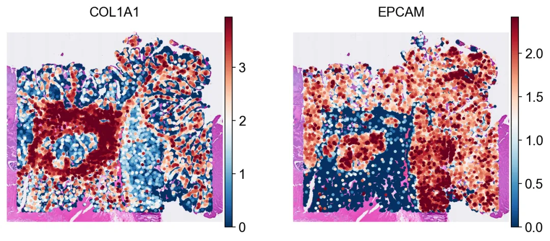 重新导入 SpaceRanger 风格目录后,细胞坐标依然能与 H&E 背景保持一致。
Cellpose 与 CellSAM 对比
CellSAM(Nature Methods 2025)是一个面向细胞分割的基础模型。为了更直观地理解不同后端之间的差异,这里在同一块 1024×1024 的组织裁剪区域上,对 Cellpose 和 CellSAM 做并排比较。
import numpy as np
import scipy.sparse, tifffile, zarr
from skimage.segmentation import find_boundaries
from omicverse.external.bin2cell import cellseg

# 从按 mpp 缩放后的 H&E 图像中读取一个 1024×1024 的裁剪区域
with tifffile.TiffFile('stardist/he_colon1.tiff') as tif:
    z = zarr.open(tif.pages[0].aszarr(), mode='r')
    h, w = z.shape[:2]
    crop = np.array(z[h//2-512:h//2+512, w//2-512:w//2+512, :3])
tifffile.imwrite('stardist/cmp_crop.tiff', crop)
print(f'Crop: {crop.shape}')
Crop: (1024, 1024, 3)
# Cellpose
cellseg('stardist/cmp_crop.tiff', 'stardist/cmp_cp.npz',
        backend='cellpose', block_size=1024, gpu=True, flow_threshold=0.4)
cp = scipy.sparse.load_npz('stardist/cmp_cp.npz').toarray()
print(f'Cellpose: {cp.max()} cells')

# CellSAM
cellseg('stardist/cmp_crop.tiff', 'stardist/cmp_cs.npz',
        backend='cellsam', block_size=1024, gpu=True)
cs = scipy.sparse.load_npz('stardist/cmp_cs.npz').toarray()
print(f'CellSAM: {cs.max()} cells')
Cellpose: 318 cells
Loading CellSAM model (cellsam_general)...
CellSAM model loaded. Image: 1024x1024
bin2cell.cellsam: 100%|██████████████████████████████████████████████████████████████████████████████████████| 1/1 [00:57<00:00, 57.57s/tile]
bin2cell.cellsam: 100%|██████████████████████████████████████████████████████████████████████████████████████| 1/1 [00:57<00:00, 57.57s/tile]
CellSAM segmentation complete: 482 cells
CellSAM: 482 cells
import matplotlib.pyplot as plt

def_overlay(ax, img, labels, title):
    ax.imshow(img)
    bnd = find_boundaries(labels, mode='outer')
    rng = np.random.RandomState(42)
    c = rng.rand(labels.max()+1, 4); c[:,3]=0.25; c[0]=[0,0,0,0]
    ax.imshow(c[labels])
    b = np.zeros((*labels.shape, 4)); b[bnd]=[0,1,0,0.8]
    ax.imshow(b)
    ax.set_title(title, fontsize=13, fontweight='bold'); ax.axis('off')

fig, axes = plt.subplots(1, 3, figsize=(18, 6))
axes[0].imshow(crop)
axes[0].set_title('H&E', fontsize=13, fontweight='bold')
axes[0].axis('off')
_overlay(axes[1], crop, cp, f'Cellpose ({cp.max()} cells)')
_overlay(axes[2], crop, cs, f'CellSAM ({cs.max()} cells)')
plt.tight_layout()
plt.show()
<Figure size 1440x480 with 3 Axes>
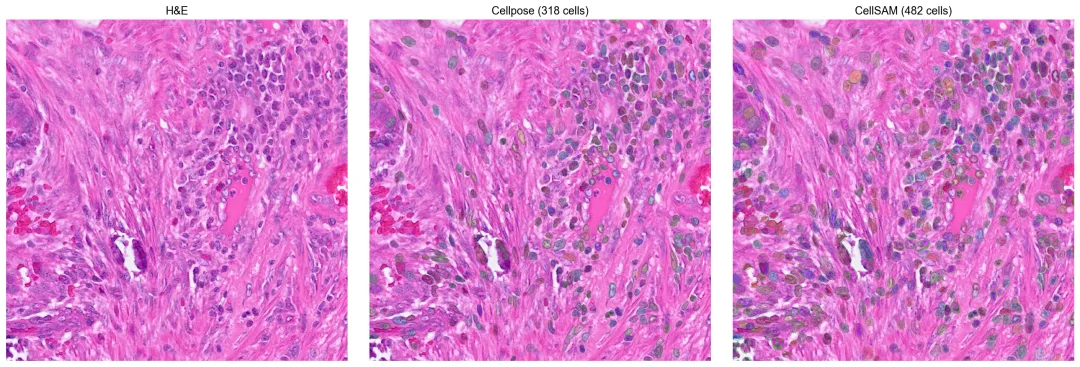 在同一块组织裁剪区域上比较 Cellpose 与 CellSAM 的分割轮廓。
细胞级空间对比
把这块 1024×1024 裁剪区域中的两套分割结果都聚合成细胞级表达对象,这样就可以在同一种空间基因表达视图下直接比较两个后端。
import numpy as np

# 为裁剪区域构建一个最小化的 bin-level adata
# 该裁剪区域在 mpp 空间中覆盖 spatial_cropped 的 [cy-512:cy+512, cx-512:cx+512]
sp = adata.obsm['spatial_cropped_150_buffer']
sample = list(adata.uns['spatial'].keys())[0]
mpp_sf = adata.uns['spatial'][sample]['scalefactors'].get(
'tissue_0.3_mpp_150_buffer_scalef', 0.91)
import tifffile
with tifffile.TiffFile('stardist/he_colon1.tiff') as t:
    h, w = t.pages[0].shape[:2]
cy, cx = h//2, w//2

# 选择在 mpp 缩放坐标下落入裁剪框内的 bin
scaled = sp * mpp_sf
cmask = ((scaled[:,1] >= cy-512) & (scaled[:,1] < cy+512) &
         (scaled[:,0] >= cx-512) & (scaled[:,0] < cx+512))
adata_sub = adata[cmask].copy()
print(f'Crop bins: {adata_sub.shape[0]}')

# Cellpose 标签已经在完整流程里写入 adata
# 这里直接基于已有的 labels_he_expanded 做 bin_to_cell
cdata_cp = ov.space.bin2cell(adata_sub, labels_key='labels_he_expanded',
                      spatial_keys=['spatial_cropped_150_buffer'])
sc.pp.normalize_total(cdata_cp); sc.pp.log1p(cdata_cp)
print(f'Cellpose cells: {cdata_cp.shape[0]}')
Crop bins: 23295
Cellpose cells: 428
# CellSAM:把裁剪区域的标签写回 adata_sub
from omicverse.external.bin2cell import insert_labels, expand_labels
import scipy.sparse

# 将 bin 的空间坐标映射到裁剪图像的像素坐标
crop_origin = np.array([cx-512, cy-512])
crop_px = (adata_sub.obsm['spatial_cropped_150_buffer'] * mpp_sf - crop_origin).astype(int)

cs_labels = scipy.sparse.load_npz('stardist/cmp_cs.npz')
lab_vals = np.zeros(len(adata_sub), dtype=int)
valid = ((crop_px[:,0] >= 0) & (crop_px[:,0] < cs_labels.shape[1]) &
         (crop_px[:,1] >= 0) & (crop_px[:,1] < cs_labels.shape[0]))
if valid.any():
    v = cs_labels[crop_px[valid,1], crop_px[valid,0]]
if scipy.sparse.issparse(v):
        v = np.asarray(v.todense()).flatten()
else:
        v = np.asarray(v).flatten()
    lab_vals[valid] = v
adata_sub.obs['labels_cellsam'] = lab_vals

expand_labels(adata_sub, labels_key='labels_cellsam',
              expanded_labels_key='labels_cellsam_exp', max_bin_distance=2)

cdata_cs = ov.space.bin2cell(adata_sub, labels_key='labels_cellsam_exp',
                      spatial_keys=['spatial_cropped_150_buffer'])
sc.pp.normalize_total(cdata_cs); sc.pp.log1p(cdata_cs)
print(f'CellSAM cells: {cdata_cs.shape[0]}')
CellSAM cells: 482
fig, axes = plt.subplots(1, 2, figsize=(14, 6))
ov.pl.spatialseg(cdata_cp, color='COL1A1', edges_color='white',
                 edges_width=0.1, alpha=0.8, ax=axes[0], show=False)
axes[0].set_title(f'Cellpose ({cdata_cp.shape[0]} cells)', fontsize=13)
ov.pl.spatialseg(cdata_cs, color='COL1A1', edges_color='white',
                 edges_width=0.1, alpha=0.8, ax=axes[1], show=False)
axes[1].set_title(f'CellSAM ({cdata_cs.shape[0]} cells)', fontsize=13)
plt.tight_layout()
plt.show()
<Figure size 1120x480 with 4 Axes>
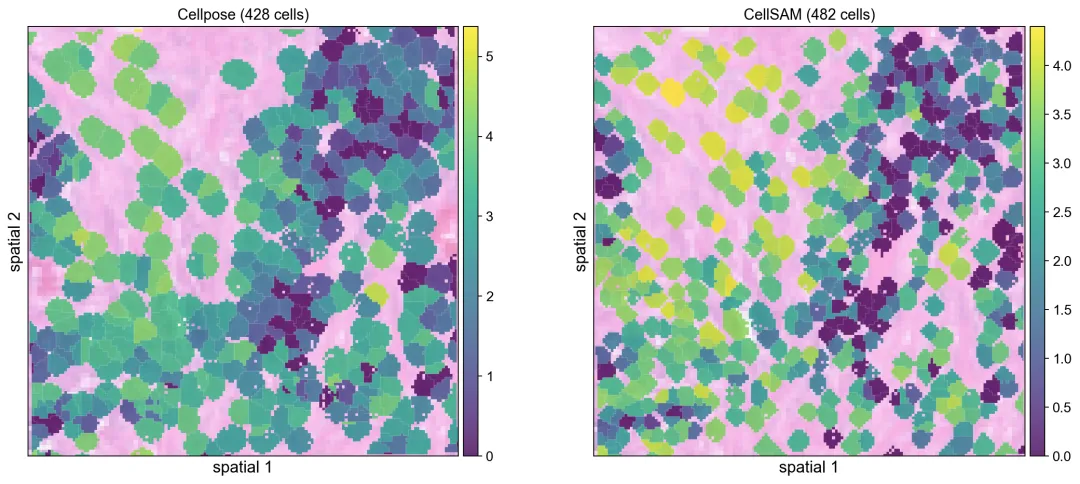 把两套分割结果聚合成细胞级表达后,可以在同一种空间视图里直接比较。
参考文献:Polański, K., Bartolomé-Casado, R., Sarropoulos, I., Xu, C., England, N., Jahnsen, F. L., ... & Yayon, N. (2024). Bin2cell reconstructs cells from high resolution Visium HD data. Bioinformatics, 40(9), btae546.
参考文献:Stringer, C., Wang, T., Michaelos, M., & Pachitariu, M. (2021). Cellpose: a generalist algorithm for cellular segmentation. Nature methods, 18(1), 100-106.

