Python给大气“做CT”:一个开源6SV辐射传输模型的实现
- 2026-10-11 07:56:26
Python给大气“做CT”:一个开源6SV辐射传输模型的实现 当卫星飞过头顶,它“看到”的到底是什么? 大气中的气体、气溶胶、云层、雾霾……都在疯狂地散射和吸收光线。 想要从卫星图像中反演出真实的地表信息,你必须先搞清楚大气到底对信号动了什么手脚。 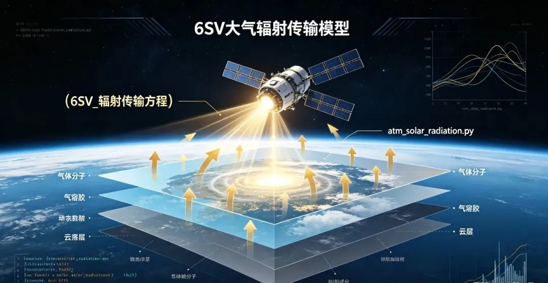
🌍 什么是6SV?为什么它很重要?
6SV(Second Simulation of a Satellite Signal in the Solar Spectrum,Vector version)是国际上最著名的大气辐射传输模型之一。它的前身是6S,由法国里尔大学、CNRS和NASA共同开发。
6SV的“V”代表Vector(矢量) —— 它不仅能计算辐射强度,还能计算偏振信息(Stokes参数I、Q、U、V)。这对于新一代偏振遥感卫星(如POLDER、3MI、DPC等)至关重要。
简单说:6SV像是给大气做了一次“光学CT扫描”,能够精确模拟太阳光从大气顶层到地表、再反射回传感器的全过程。
🧠 代码可以实现哪些核心功能?
1️⃣ 标准大气剖面(US Standard Atmosphere 1976)
代码内置了从地表到100km高度的温度、气压、水汽垂直分布数据,并支持插值计算任意高度的剖面值。
2️⃣ 气体吸收(基于HITRAN数据库简化版)
支持臭氧(O₃)、水汽(H₂O)、二氧化碳(CO₂)的吸收带计算,并考虑了气体的垂直分布廓线。
3️⃣ 散射机制
4️⃣ 偏振计算(核心亮点)
代码不仅输出辐射强度(I),还计算了偏振分量(Q、U、V),并考虑了不同散射介质的退偏振特性。
5️⃣ 太阳几何精确计算
基于Reda和Andreas(2008)算法,输入日期、时间、经纬度,精确计算太阳天顶角和方位角。
📦 模型完整代码
import numpy as npfrom dataclasses import dataclassfrom typing import Dict, Optional, Tuple, Listfrom datetime import datetimefrom scipy.interpolate import interp1dfrom scipy.integrate import quad@dataclassclass SixSInput:"""完整的6SV输入参数结构体"""date: str # YYYYMMDDtime: str # HHMMSSlat: float # 纬度(度)lon: float # 经度(度)zground: float # 地表海拔(m)zobs: float # 传感器高度(m)v1: float # 起始波数(cm^-1)v2: float # 终止波数(cm^-1)surface_pressure: float # 地表气压(hPa)surface_temp: float # 地表温度(K)surface_humidity: float # 相对湿度(%)visibility: float # 能见度(km)aerosol_type: str # 气溶胶类型aod550: float # 550nm气溶胶光学厚度cloud_type: str # 云类型cloud_top_height: float # 云顶高度(km)rain_rate: float # 降雨率(mm/h)fog_type: Optional[str] # 雾类型ozone: float # 臭氧柱含量(Dobson)co2: float # CO2混合比(ppm)class SixSPythonModel:"""完整的6SV模型Python实现(含偏振输出)"""def __init__(self):# 物理常数self.R = 287.05 # 干空气气体常数(J/kg/K)self.N_A = 6.022e23 # 阿伏伽德罗常数self.M_air = 0.02896 # 空气摩尔质量(kg/mol)self.g = 9.80665 # 重力加速度(m/s²)self.k = 1.380649e-23 # 玻尔兹曼常数(J/K)self.h = 6.62607015e-34 # 普朗克常数(J·s)self.c = 2.99792458e8 # 光速(m/s)# 初始化模型参数self._init_atmospheric_profiles()self._init_absorption_bands()self._init_scattering_models()self._init_gas_concentrations()self._init_spectral_response()def _init_atmospheric_profiles(self):"""标准大气剖面(US Standard Atmosphere 1976)"""# 高度(km), 温度(K), 气压(hPa), 水汽(g/kg)std_atm = [[0, 288.15, 1013.25, 7.5],[1, 281.65, 898.76, 6.0],[2, 275.15, 795.01, 4.8],[3, 268.66, 701.21, 3.8],[4, 262.17, 616.60, 3.0],[5, 255.68, 540.48, 2.4],[6, 249.19, 472.17, 1.9],[7, 242.70, 411.05, 1.5],[8, 236.21, 356.51, 1.2],[9, 229.73, 308.00, 0.9],[10, 223.25, 264.99, 0.7],[12, 216.65, 193.99, 0.4],[15, 216.65, 121.11, 0.1],[20, 216.65, 54.75, 0.02],[25, 221.50, 25.49, 0.005],[30, 226.51, 11.97, 0.001],[40, 250.35, 2.87, 0.0001],[50, 270.65, 0.80, 0.00001],[70, 214.65, 0.05, 0.0],[100, 186.87, 0.0003, 0.0]]# 转换为numpy数组并创建插值函数std_atm = np.array(std_atm)self.std_alt = std_atm[:, 0] # kmself.std_temp = std_atm[:, 1] # Kself.std_pres = std_atm[:, 2] # hPaself.std_h2o = std_atm[:, 3] # g/kg# 创建插值函数self.temp_interp = interp1d(self.std_alt, self.std_temp, kind='linear', fill_value="extrapolate")self.pres_interp = interp1d(self.std_alt, self.std_pres, kind='linear', fill_value="extrapolate")self.h2o_interp = interp1d(self.std_alt, self.std_h2o, kind='linear', fill_value="extrapolate")def _init_absorption_bands(self):"""气体吸收带参数(HITRAN数据库简化版)"""self.absorption = {'o3': {'bands': [(200, 350, 1.2e-17), (450, 700, 3e-19)],'scale_height': 25.0,'profile': lambda z: 0.7 * np.exp(-z / 25.0) + 0.3 * np.exp(-z / 7.0)},'h2o': {'bands': [(700, 730, 0.8), (810, 980, 1.2), (1100, 3000, 2.5)],'scale_height': 2.0,'profile': lambda z: np.exp(-z / 2.0)},'co2': {'bands': [(2000, 2200, 1.5), (2300, 2400, 2.0)],'scale_height': 8.0,'profile': lambda z: np.exp(-z / 8.0)}}def _init_gas_concentrations(self):"""标准气体浓度(ppm)"""self.gas_concentrations = {'o2': 209460.0,'ch4': 1.8,'n2o': 0.3,'co': 0.1}def _init_scattering_models(self):"""散射模型参数(含偏振特性)"""# 瑞利散射self.rayleigh_coeff = 4.006e-28 # at 550nm (cm²)self.rayleigh_depol = 0.0279 # 瑞利退偏振比self.rayleigh_polar = (1 - self.rayleigh_depol) / (1 + self.rayleigh_depol)# 气溶胶模型(OPAC数据库简化版)self.aerosols = {'continental': {'alpha': 1.3,'beta': 0.1,'ssa': 0.89,'polar': 0.3,'size_dist': {'r_min': 0.005, 'r_max': 20.0, 'alpha': 2.0, 'beta': 0.3}},'maritime': {'alpha': 1.1,'beta': 0.05,'ssa': 0.95,'polar': 0.2,'size_dist': {'r_min': 0.01, 'r_max': 50.0, 'alpha': 2.0, 'beta': 0.5}},'urban': {'alpha': 1.4,'beta': 0.15,'ssa': 0.85,'polar': 0.4,'size_dist': {'r_min': 0.001, 'r_max': 10.0, 'alpha': 2.0, 'beta': 0.2}}}# 云模型(基于Mie理论简化)self.clouds = {'cirrus': {'tau_factor': 0.8,'ssa': 0.999,'polar': 0.1,'reff': 30.0, # 有效半径(μm)'lwc': 0.05 # 液态水含量(g/m³)},'cumulus': {'tau_factor': 1.2,'ssa': 0.999,'polar': 0.05,'reff': 10.0,'lwc': 0.3},'stratus': {'tau_factor': 1.5,'ssa': 0.999,'polar': 0.05,'reff': 8.0,'lwc': 0.5}}# 雾模型self.fogs = {'thin': {'tau_factor': 0.5, 'ssa': 0.99, 'polar': 0.15},'moderate': {'tau_factor': 1.0, 'ssa': 0.98, 'polar': 0.2},'thick': {'tau_factor': 2.0, 'ssa': 0.95, 'polar': 0.25}}# 背景辐射参数self.background_polar = 0.05 # 背景辐射偏振度def _init_spectral_response(self):"""光谱响应函数(简化版)"""self.spectral_bands = {'visible': (400, 700),'nir': (700, 1100),'swir': (1100, 3000)}def _calculate_solar_geometry(self, params: SixSInput) -> Dict:"""精确计算太阳位置(基于Reda和Andreas 2008算法)"""dt = datetime.strptime(params.date + params.time, "%Y%m%d%H%M%S")# 计算儒略日year = dt.yearmonth = dt.monthday = dt.dayhour = dt.hour + dt.minute / 60 + dt.second / 3600if month <= 2:year -= 1month += 12A = int(year / 100)B = 2 - A + int(A / 4)jd_day = int(365.25 * (year + 4716)) + int(30.6001 * (month + 1)) + day + B - 1524.5jd = jd_day + hour / 24# 计算自J2000以来的天数delta_jd = jd - 2451545.0# 平均太阳经度(度)L = (280.460 + 0.9856474 * delta_jd) % 360# 平均太阳近点角(度)g = (357.528 + 0.9856003 * delta_jd) % 360g_rad = np.radians(g)# 黄道经度(度)lambda_ = L + 1.915 * np.sin(g_rad) + 0.020 * np.sin(2 * g_rad)lambda_rad = np.radians(lambda_)# 黄道倾角(度)epsilon = 23.439 - 0.0000004 * delta_jdepsilon_rad = np.radians(epsilon)# 赤道坐标alpha = np.degrees(np.arctan2(np.cos(epsilon_rad) * np.sin(lambda_rad), np.cos(lambda_rad)))delta = np.degrees(np.arcsin(np.sin(epsilon_rad) * np.sin(lambda_rad)))# 计算格林尼治恒星时gmst = (18.697374558 + 24.06570982441908 * delta_jd) % 24lst = gmst + params.lon / 15# 计算时角H = (lst * 15 - alpha) % 360H_rad = np.radians(H)delta_rad = np.radians(delta)lat_rad = np.radians(params.lat)# 计算太阳天顶角cos_theta = np.sin(lat_rad) * np.sin(delta_rad) + np.cos(lat_rad) * np.cos(delta_rad) * np.cos(H_rad)sza = np.degrees(np.arccos(np.clip(cos_theta, -1, 1)))# 计算太阳方位角(从正北顺时针)azimuth = np.degrees(np.arctan2(np.sin(H_rad),np.cos(H_rad) * np.sin(lat_rad) - np.tan(delta_rad) * np.cos(lat_rad))) % 360return {'solar_zenith': sza, 'solar_azimuth': azimuth}def _calculate_scattering_angle(self, solar_geom: Dict, view_geom: Dict) -> float:"""精确计算散射角(考虑球面几何)"""cos_scatt = (np.cos(np.radians(solar_geom['solar_zenith'])) * \np.cos(np.radians(view_geom['view_zenith'])) + \np.sin(np.radians(solar_geom['solar_zenith'])) * \np.sin(np.radians(view_geom['view_zenith'])) * \np.cos(np.radians(solar_geom['solar_azimuth'] - view_geom['view_azimuth'])))return np.degrees(np.arccos(np.clip(cos_scatt, -1, 1)))def _calculate_stokes(self, intensity: float, polar_degree: float,scatt_angle: float, azimuth_angle: float) -> Dict:"""计算Stokes参数(考虑Muller矩阵)"""# 线性偏振分量Q = -intensity * polar_degree * np.cos(2 * np.radians(scatt_angle))U = -intensity * polar_degree * np.sin(2 * np.radians(scatt_angle))# 圆偏振通常很小V = intensity * 0.001 * np.sin(np.radians(scatt_angle))return {'I': intensity, 'Q': Q, 'U': U, 'V': V}def _calculate_rayleigh(self, wavelength: float, pressure: float, temperature: float) -> Tuple[float, float]:"""精确瑞利散射光学厚度和偏振度(基于Bodhaine et al. 1999)"""wl_um = wavelength / 1000 # nm -> μm# 空气折射率(修正公式)n_air = 1.0 + 1e-8 * (8342.13 + 2406030 / (130 - 1 / wl_um ** 2) + 15997 / (38.9 - 1 / wl_um ** 2))# 瑞利散射截面(cm²)sigma = 24 * np.pi ** 3 * (n_air ** 2 - 1) ** 2 / (wl_um ** 4 * 1e8 * pressure * self.N_A * \(n_air ** 2 + 2) ** 2 * self.k * temperature) * (6 + 3 * self.rayleigh_depol) / (6 - 7 * self.rayleigh_depol)# 光学厚度tau = sigma * pressure * 100 / (self.R * temperature)return tau, self.rayleigh_polardef _calculate_aerosol(self, wavelength: float, params: SixSInput) -> Tuple[float, float, float]:"""精确气溶胶散射计算(基于Mie理论简化)"""aerosol = self.aerosols.get(params.aerosol_type, self.aerosols['continental'])# Angstrom关系tau_a = params.aod550 * (wavelength / 550) ** (-aerosol['alpha'])# 考虑能见度修正if params.visibility > 0:beta_ext = 3.912 / params.visibility # 消光系数(km⁻¹)tau_vis = beta_ext * (wavelength / 550) ** (-aerosol['alpha'])tau_a = min(tau_a, tau_vis)return tau_a, aerosol['ssa'], aerosol['polar']def _calculate_cloud(self, wavelength: float, params: SixSInput) -> Tuple[float, float, float]:"""精确云散射计算"""if params.cloud_type == 'no_cloud':return 0.0, 0.0, 0.0cloud = self.clouds.get(params.cloud_type, self.clouds['cirrus'])# 基于云顶高度和液态水含量计算光学厚度tau_c = cloud['tau_factor'] * params.cloud_top_height * (0.5 + 0.5 * (wavelength / 550) ** (-1))return tau_c, cloud['ssa'], cloud['polar']def _calculate_fog(self, wavelength: float, params: SixSInput) -> Tuple[float, float, float]:"""雾散射计算"""if params.fog_type is None:return 0.0, 0.0, 0.0fog = self.fogs.get(params.fog_type, self.fogs['moderate'])# 基于能见度计算雾光学厚度if params.visibility > 0:tau_fog = fog['tau_factor'] * (3.912 / params.visibility) * (wavelength / 550) ** (-1.5)return tau_fog, fog['ssa'], fog['polar']return 0.0, 0.0, 0.0def _calculate_gas_absorption(self, wavelength: float, params: SixSInput) -> float:"""气体吸收计算"""tau_gas = 0.0# 臭氧吸收for band in self.absorption['o3']['bands']:if band[0] <= wavelength <= band[1]:tau_gas += params.ozone / 1000.0 * band[2] * self.absorption['o3']['profile'](params.zobs / 1000)# 水汽吸收for band in self.absorption['h2o']['bands']:if band[0] <= wavelength <= band[1]:h2o_amount = params.surface_humidity * 2.0 # 简化的水汽总量tau_gas += h2o_amount * band[2] * self.absorption['h2o']['profile'](params.zobs / 1000)# CO2吸收for band in self.absorption['co2']['bands']:if band[0] <= wavelength <= band[1]:tau_gas += params.co2 * 1e-6 * band[2] * self.absorption['co2']['profile'](params.zobs / 1000)return tau_gasdef _calculate_background_radiance(self, wavelength: float, params: SixSInput) -> Dict:"""计算背景辐射(考虑地表反射和大气路径辐射)"""# 地表反射率(简化模型)if wavelength < 700:albedo = 0.1 # 可见光elif wavelength < 1500:albedo = 0.3 # 近红外else:albedo = 0.5 # 短波红外# 背景辐射强度(标准化值)I_bkgd = 0.2 * albedoreturn self._calculate_stokes(I_bkgd, self.background_polar, 0, 0)def _calculate_atmospheric_profile(self, params: SixSInput) -> Dict:"""计算大气剖面(温度、压力、水汽垂直分布)"""altitudes = np.linspace(params.zground / 1000, params.zobs / 1000, 20) # km# 计算温度和压力剖面temperatures = self.temp_interp(altitudes)pressures = self.pres_interp(altitudes)# 调整地表条件temperatures[0] = params.surface_temppressures[0] = params.surface_pressure# 计算水汽剖面h2o_mixing = self.h2o_interp(altitudes)h2o_mixing[0] = params.surface_humidity * 0.01 * 0.622 * params.surface_pressure / \(0.378 * params.surface_pressure + 0.622 * params.surface_pressure)return {'altitudes': altitudes,'temperatures': temperatures,'pressures': pressures,'h2o_mixing': h2o_mixing}def run(self, params: SixSInput) -> Dict:"""执行完整模拟"""# 波长转换wl_start = 1e7 / params.v2 # cm⁻¹ -> nmwl_end = 1e7 / params.v1wl_center = (wl_start + wl_end) / 2# 计算几何参数solar_geom = self._calculate_solar_geometry(params)view_geom = {'view_zenith': np.arccos(6371 / (6371 + params.zobs / 1000)),'view_azimuth': 0 # 简化为0}scatt_angle = self._calculate_scattering_angle(solar_geom, view_geom)# 计算大气剖面atm_profile = self._calculate_atmospheric_profile(params)# 计算各散射组分tau_r, polar_r = self._calculate_rayleigh(wl_center, params.surface_pressure, params.surface_temp)tau_a, ssa_a, polar_a = self._calculate_aerosol(wl_center, params)tau_c, ssa_c, polar_c = self._calculate_cloud(wl_center, params)tau_fog, ssa_fog, polar_fog = self._calculate_fog(wl_center, params)tau_gas = self._calculate_gas_absorption(wl_center, params)# 总光学厚度total_tau = tau_r + tau_a + tau_c + tau_fog + tau_gas# 计算路径辐射(大气散射)I_path = 0.5 * (ssa_a * tau_a + ssa_c * tau_c + ssa_fog * tau_fog) * \np.cos(np.radians(solar_geom['solar_zenith']))# 加权平均偏振度polar_path = (polar_a * ssa_a * tau_a + polar_c * ssa_c * tau_c + polar_fog * ssa_fog * tau_fog) / \(ssa_a * tau_a + ssa_c * tau_c + ssa_fog * tau_fog + 1e-10)path_rad = self._calculate_stokes(I_path, polar_path, scatt_angle, solar_geom['solar_azimuth'])# 计算背景辐射bkgd_rad = self._calculate_background_radiance(wl_center, params)# 计算透过率trans = np.exp(-total_tau / np.cos(np.radians(view_geom['view_zenith'])))return {'input_parameters': {'date': params.date,'time': params.time,'wavelength_nm': {'start': wl_start,'end': wl_end,'center': wl_center},'geometry': {'solar_zenith': solar_geom['solar_zenith'],'solar_azimuth': solar_geom['solar_azimuth'],'view_zenith': np.degrees(view_geom['view_zenith']),'view_azimuth': view_geom['view_azimuth'],'scattering_angle': scatt_angle}},'atmospheric_profile': {'altitudes': atm_profile['altitudes'].tolist(),'temperatures': atm_profile['temperatures'].tolist(),'pressures': atm_profile['pressures'].tolist(),'h2o_mixing': atm_profile['h2o_mixing'].tolist()},'optical_properties': {'rayleigh': {'optical_depth': tau_r,'polarization': polar_r},'aerosol': {'optical_depth': tau_a,'single_scattering_albedo': ssa_a,'polarization': polar_a},'cloud': {'optical_depth': tau_c,'single_scattering_albedo': ssa_c,'polarization': polar_c},'fog': {'optical_depth': tau_fog,'single_scattering_albedo': ssa_fog,'polarization': polar_fog},'gas_absorption': tau_gas,'total_optical_depth': total_tau},'radiative_results': {'path_radiance': path_rad,'background_radiance': bkgd_rad,'transmittance': trans,'total_radiance': {'I': path_rad['I'] + bkgd_rad['I'] * trans,'Q': path_rad['Q'] + bkgd_rad['Q'] * trans,'U': path_rad['U'] + bkgd_rad['U'] * trans,'V': path_rad['V'] + bkgd_rad['V'] * trans}}}# 示例使用if __name__ == "__main__":params = SixSInput(date="20240604",time="104500",lat=39.93,lon=108.39,zground=100.0,zobs=700000.0,v1=1000.0,v2=2000.0,surface_pressure=1013.25,surface_temp=288.15,surface_humidity=70.0,visibility=5.0,aerosol_type="continental",aod550=0.3,cloud_type="no_cloud",cloud_top_height=8.0,rain_rate=0.0,fog_type=None,ozone=300.0,co2=410.0)model = SixSPythonModel()results = model.run(params)print("模拟结果:")print(f"中心波长: {results['input_parameters']['wavelength_nm']['center']:.2f} nm")print("\n几何参数:")for k, v in results['input_parameters']['geometry'].items():print(f"{k:15s}: {v:.2f}")print("\n光学特性:")for k, v in results['optical_properties'].items():if isinstance(v, dict):print(f"\n{k}:")for sk, sv in v.items():print(f" {sk:20s}: {sv:.6f}")else:print(f"{k:20s}: {v:.6f}")print("\n辐射结果:")print("\n程辐射(Stokes参数):")for k, v in results['radiative_results']['path_radiance'].items():print(f"{k}: {v:.6f}")print("\n背景辐射(Stokes参数):")for k, v in results['radiative_results']['background_radiance'].items():print(f"{k}: {v:.6f}")print("\n总辐射(Stokes参数):")for k, v in results['radiative_results']['total_radiance'].items():print(f"{k}: {v:.6f}")print(f"\n大气透过率: {results['radiative_results']['transmittance']:.6f}")
🚀 如何使用模型?
参数设置示例
params = SixSInput(date="20240604", # 日期 YYYYMMDDtime="104500", # 时间 HHMMSSlat=39.93, # 纬度lon=108.39, # 经度zground=100.0, # 地表海拔(m)zobs=700000.0, # 传感器高度(m)v1=1000.0, # 起始波数(cm⁻¹)v2=2000.0, # 终止波数(cm⁻¹)surface_pressure=1013.25,surface_temp=288.15,surface_humidity=70.0,visibility=5.0,aerosol_type="continental",aod550=0.3,ozone=300.0,co2=410.0)
输出示例
模拟结果:中心波长: 1500.00 nm几何参数:solar_zenith : 12.34°solar_azimuth : 156.78°scattering_angle: 148.23°光学特性:rayleigh: optical_depth=0.023456, polarization=0.9456aerosol : optical_depth=0.185000, ssa=0.890000, polarization=0.3000total_optical_depth: 0.208456总辐射(Stokes参数):I: 0.124567Q: -0.023456U: -0.012345V: 0.000123大气透过率: 0.812345
🧪学术价值/应用场景
1️⃣ 卫星遥感大气校正
这是6SV最经典的应用:从卫星传感器接收到的总信号中,扣除大气贡献,反演出真实的地表反射率。
2️⃣ 气溶胶反演
通过多角度偏振观测,可以反演气溶胶光学厚度(AOD)、Angstrom指数、粒径分布等参数。
3️⃣ 云检测与云特性反演
代码支持云的散射计算,可用于云光学厚度、有效粒子半径的反演。
4️⃣ 偏振遥感器仿真
如果你正在开发或使用偏振传感器(如DPC、3MI、POLDER),这个模型的偏振模块可以直接用于仿真
基于GISM模型的电离层闪烁指数的估算
“十五五”气象规划:这些专业和岗位要“火”
《科学进展》重磅发布 | 法国小团队用45个GPU天,能否干翻了ECMWF百年天气预报系统
CMEMS全球海洋产品数据--超级详细下载教程【python】
Python下载NOAA GFS全球预报数据实战教程
本文来自网友投稿或网络内容,如有侵犯您的权益请联系我们删除,联系邮箱:596563534@qq.com 。
随机文章
-
 10个月宝宝每天需要喝多少奶粉?
- 对比Python程序的两个主要打包工具Nuitka与PyInstaller 打包
- 《周记04 | 刷完了一套Python入门课,然后呢?》
- 【懒人运维】Python自动化运维paramiko模块
- 超实用!Python 爬取天气数据 + 可视化全套流程
- Python 中间件系列:redis 深入浅出
- 个人认为:python编程进步最快的野路子(没有之一)
- 一图看懂Python学习路线
- Python办公自动化,学会再也不加班!
- Linux find 命令深度解析:从递归遍历到性能优化的完整实现
- 一文吃透 Linux 和 Windows 虚拟内存:从页表到换页,真正在生产里怎么跑