基于MNE Python进行空间信号分离(SSS)及Maxwellfiltering——MEG分析必看
- 2026-10-11 06:41:11

本教程参考https://mne.tools/stable/auto_tutorials/preprocessing/60_maxwell_filtering_sss.html?utm_source=chatgpt.com#caveats-to-using-sss-maxwell-filtering
可在茗创科技公众号后台回复关键词MEG_SSS获取代码
SSS 和 Maxwell filtering 的背景
SSS(Signal-Space Separation,信号空间分离)是一种基于电磁场物理学的技术。它会把 MEG 测量到的信号分解成两部分:一部分来自传感器阵列内部,也就是脑内的信号(internal components);另一部分来自传感器阵列外部,也就是环境中的磁噪声(external components)。由于这两部分在数学上是线性独立的,因此可以通过去掉外部成分减少数据中的环境噪声。Maxwell filtering(Maxwell 滤波)是与 SSS 相关的一种处理方法,它会进一步去除内部子空间中的高阶成分(这些高阶成分通常主要由传感器噪声主导)。通常情况下,SSS 和 Maxwell filtering 会一起使用,在 MNE-Python 中,它们被实现为同一个函数。
需要注意的是,Maxwell filtering 最初是为 Elekta Neuromag 系统开发,因此对于非 Neuromag 的 MEG 数据,目前仍应视为实验性方法。具体请参阅maxwell_filter() 函数文档中的注释。
一、载入处理模块并加载示例数据,并对数据进行裁剪以节省内存
import osimport matplotlib.pyplot as pltimport numpy as npimport pandas as pdimport seaborn as snsimport mnefrom mne.preprocessing import find_bad_channels_maxwellsample_data_folder = mne.datasets.sample.data_path()sample_data_raw_file = os.path.join( sample_data_folder, "MEG", "sample", "sample_audvis_raw.fif")raw = mne.io.read_raw_fif(sample_data_raw_file, verbose=False)raw.crop(tmax=60)MNE-Python 中实现的 SSS / Maxwell filtering 目前提供以下功能:
- 基础坏通道检测(
find_bad_channels_maxwell()) - 坏通道重建
- 串扰(cross-talk)消除
- 精细校准(fine calibration)校正
- tSSS(temporal SSS)
- 坐标系转换
- 使用信息论对内部成分进行正则化
- 原始数据的头动补偿(利用 MaxFilter 估计的头位置信息)
- cHPI 信号去除(见
mne.chpi.filter_chpi()) - 支持 3D 精细校准文件(不包括1D)
- 基于 epoch 的头动补偿(通过
mne.epochs.average_movements()实现) - 对非 Elekta 系统数据提供实验性的处理支持(未进行 movement compensation 的数据)
二、载入fine calibration file(精细校准文件)及crosstalk compensation file(串扰补偿文件)——选做
fine_cal_file = os.path.join(sample_data_folder, "SSS", "sss_cal_mgh.dat")crosstalk_file = os.path.join(sample_data_folder, "SSS", "ct_sparse_mgh.fif")三、标记坏通道,此步一定要在空间重建之前
先进行自动检测坏通道(本次数据中通道MEG2443噪声较大)
raw.info["bads"] = []raw_check = raw.copy()auto_noisy_chs, auto_flat_chs, auto_scores = find_bad_channels_maxwell( raw_check, cross_talk=crosstalk_file, calibration=fine_cal_file, return_scores=True, verbose=True,)print(auto_noisy_chs) # we should find them!print(auto_flat_chs) # none for this dataset将会输出:
Applying low-pass filter with 40.0 Hz cutoff frequency ...Reading 0 ... 36037 = 0.000 ... 60.000 secs...Filtering raw data in 1 contiguous segmentSetting up low-pass filter at 40 HzFIR filter parameters---------------------Designing a one-pass, zero-phase, non-causal lowpass filter:- Windowed time-domain design (firwin) method- Hamming window with 0.0194 passband ripple and 53 dB stopband attenuation- Upper passband edge: 40.00 Hz- Upper transition bandwidth: 10.00 Hz (-6 dB cutoff frequency: 45.00 Hz)- Filter length: 199 samples (0.331 s)Scanning for bad channels in 12 intervals (5.0 s) ... No bad MEG channels Processing 204 gradiometers and 102 magnetometers Using fine calibration sss_cal_mgh.dat Adjusting non-orthogonal EX and EY Adjusted coil orientations by (μ ± σ): 0.5° ± 0.4° (max: 2.1°) Automatic origin fit: head of radius 91.2 mm Using origin -4.2, 16.4, 51.8 mm in the head frame Interval 1: 0.000 - 4.998 Interval 2: 5.000 - 9.998 Interval 3: 10.000 - 14.998 Interval 4: 15.000 - 19.998 Interval 5: 20.000 - 24.998 Interval 6: 24.999 - 29.998 Interval 7: 29.999 - 34.997 Interval 8: 34.999 - 39.997 Interval 9: 39.999 - 44.997 Interval 10: 44.999 - 49.997 Interval 11: 49.999 - 54.997 Interval 12: 54.999 - 60.000 Static bad channels: ['MEG 2443'] Static flat channels: [][done]['MEG 2443'][]注意find_bad_channels_maxwell函数需要输入的是没有工频噪声、cHPI信号的干净数据。默认会进行40 Hz 低通滤波。
将检测到的坏通道更新至数据中
bads = raw.info["bads"] + auto_noisy_chs + auto_flat_chsraw.info["bads"] = bads可视化自动检测坏通道的评分结果,方便后续人工检查
# Only select the data for gradiometer channels.ch_type = "grad"ch_subset = auto_scores["ch_types"] == ch_typech_names = auto_scores["ch_names"][ch_subset]scores = auto_scores["scores_noisy"][ch_subset]limits = auto_scores["limits_noisy"][ch_subset]bins = auto_scores["bins"] # The the windows that were evaluated.# We will label each segment by its start and stop time, with up to 3# digits before and 3 digits after the decimal place (1 ms precision).bin_labels = [f"{start:3.3f} – {stop:3.3f}" for start, stop in bins]# We store the data in a Pandas DataFrame. The seaborn heatmap function# we will call below will then be able to automatically assign the correct# labels to all axes.data_to_plot = pd.DataFrame( data=scores, columns=pd.Index(bin_labels, name="Time (s)"), index=pd.Index(ch_names, name="Channel"),)# First, plot the "raw" scores.fig, ax = plt.subplots(1, 2, figsize=(12, 8), layout="constrained")fig.suptitle( f"Automated noisy channel detection: {ch_type}", fontsize=16, fontweight="bold")sns.heatmap(data=data_to_plot, cmap="Reds", cbar_kws=dict(label="Score"), ax=ax[0])[ ax[0].axvline(x, ls="dashed", lw=0.25, dashes=(25, 15), color="gray") for x in range(1, len(bins))]ax[0].set_title("All Scores", fontweight="bold")# Now, adjust the color range to highlight segments that exceeded the limit.sns.heatmap( data=data_to_plot, vmin=np.nanmin(limits), # bads in input data have NaN limits cmap="Reds", cbar_kws=dict(label="Score"), ax=ax[1],)[ ax[1].axvline(x, ls="dashed", lw=0.25, dashes=(25, 15), color="gray") for x in range(1, len(bins))]ax[1].set_title("Scores > Limit", fontweight="bold")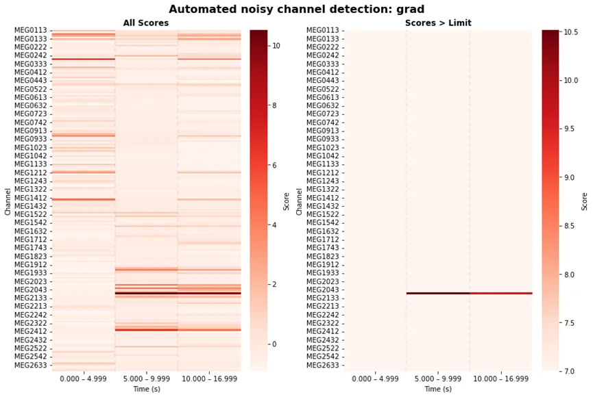
生成了一张原始评分图像及阈值化后评分,辅助进行人工检查。
自动化方法并不完美,最好同步进行人工检查,标记坏通道。
如下语句为增加人工检查后添加标记MEG2313为坏通道
raw.info["bads"] += ["MEG 2313"] # from manual inspection四、调用函数对数据进行SSS 与 Maxwell filtering
raw_sss = mne.preprocessing.maxwell_filter( raw, cross_talk=crosstalk_file, calibration=fine_cal_file, verbose=True)运行该函数将会输出如下信息,且先前标记的两个坏通道将在此步被修复(后续无需插值矫正)
Maxwell filtering raw data Bad MEG channels being reconstructed: ['MEG 2443', 'MEG 2313'] Processing 204 gradiometers and 102 magnetometers Using fine calibration sss_cal_mgh.dat Adjusting non-orthogonal EX and EY Adjusted coil orientations by (μ ± σ): 0.5° ± 0.4° (max: 2.1°) Automatic origin fit: head of radius 91.2 mm Using origin -4.2, 16.4, 51.8 mm in the head frame Loading raw data from disk Using 87/95 harmonic components for 0.000 (72/80 in, 15/15 out) Processing 6 data chunks of (at least) 10.0 s with 0.0 s overlap and boxcar windowing The final 0.0033299202193064646 s will be lumped into the final window Using 87/95 harmonic components for 0.000 (72/80 in, 15/15 out)[done]可以可视化具体效果
raw.pick(["meg"]).plot(duration=2, butterfly=True)raw_sss.pick(["meg"]).plot(duration=2, butterfly=True)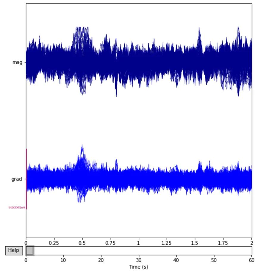
五、头动矫正
如果拥有被试头部相对于MEG传感器的位置变化信息,那么 SSS 在进行信号重建时可以把头动因素考虑进去,从而减少头部运动对 MEG 数据的影响。这里提到的头位置信息通常来自 cHPI(continuous Head Position Indicator,连续头位置指示线圈)。这些小线圈会固定在受试者头上,并以特定频率持续发射磁信号,MEG 系统便可以实时追踪头部位置变化。
chpi_fif_file = os.path.join( mne.datasets.testing.data_path(), "SSS", "test_move_anon_raw.fif")raw = mne.io.read_raw_fif(chpi_fif_file, allow_maxshield="yes")# time-resolved information on active HPI coils# if all hpi were inactive n_active is a zero-arrayn_active = mne.chpi.get_active_chpi(raw)print(f"Average number of coils active during recording: {n_active.mean()}")将会输出如下信息,检测到5个cHPI线圈都在正常工作
Opening raw data file /home/circleci/mne_data/MNE-testing-data/SSS/test_move_anon_raw.fif... Read a total of 12 projection items: mag.fif : PCA-v1 (1 x 306) idle mag.fif : PCA-v2 (1 x 306) idle mag.fif : PCA-v3 (1 x 306) idle mag.fif : PCA-v4 (1 x 306) idle mag.fif : PCA-v5 (1 x 306) idle mag.fif : PCA-v6 (1 x 306) idle mag.fif : PCA-v7 (1 x 306) idle grad.fif : PCA-v1 (1 x 306) idle grad.fif : PCA-v2 (1 x 306) idle grad.fif : PCA-v3 (1 x 306) idle grad.fif : PCA-v4 (1 x 306) idle Average EEG reference (1 x 60) idle Range : 10800 ... 31199 = 9.000 ... 25.999 secsReady.Using 5 HPI coils: 83 143 203 263 323 HzAverage number of coils active during recording: 5.0查看头部运动轨迹,检测是否有头动严重的被试或者时间段。
head_pos_file = os.path.join( mne.datasets.testing.data_path(), "SSS", "test_move_anon_raw.pos")head_pos = mne.chpi.read_head_pos(head_pos_file)mne.viz.plot_head_positions(head_pos, mode="traces")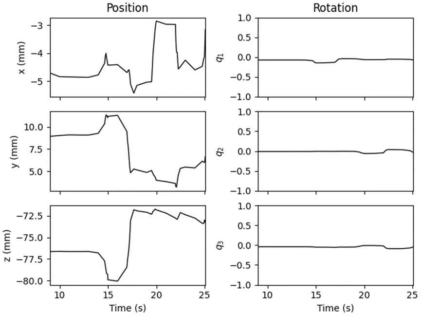
脑电数据分析启航班(训练营:2026.6.5~7.4)
核磁培训班
磁共振弥散张量成像(DTI)数据处理班(训练营:2026.7.2~7.10,新增DTI-ALPS)
磁共振弥散张量成像(DTI)数据处理进阶班(训练营:2026.7.13~7.24,新增GBSS实操内容)
多模态脑网络数据处理进阶班(训练营:2026.7.6~7.18,新增共激活模式分析)
MATLAB脑影像机器学习(直播:2026.5.26~6.18)
专题班系列
基于皮层的功能像磁共振分析专题班(训练营:2026.7.16~7.25)
1v1全程陪跑磁共振弥散张量成像(DTI)进阶数据处理教学服务
1v1全程陪跑新生儿磁共振扩散加权成像(DWI)数据处理教学服务
一对一脑电数据分析面授班(长沙:2026.6.8~6.12)
会员系列
相关说明
本文内容仅供参考。
非常欢迎大家留言、转载、收藏或分享~
本文来自微信公众号“茗创科技”。如需转载,请在“茗创科技”后台回复“转载”,并附上所需转载的文章标题以及您的ID。
茗创科技
MC_Brain
觉得有帮助,欢迎转发收藏或者点个在看哦~
听说点在看的人SCI接收率都提升了18%呢!
随机文章
-
 10个月宝宝每天需要喝多少奶粉?
- Linux I/O 子系统整体架构解析:从用户空间到硬件设备的数据通路
- 架构演进:从Python到Node.js——公众号中转站的技术选型之路
- 学习QMT股票量化系统:用python写一个简单的策略——多因子选股(附带完整源代码)
- 10天掌握Python基础语法!(第1-5天)
- 一次真实的 Linux 应急响应处置过程
- HyperMesh Python 二次开发 提高脚本运行速度的方法(以每个solid建立一个component为例)
- nicegui:简单易用的 Python UI 框架
- Python-26-(宽表和长表互换)
- Python四大免费爬虫网站
- RK3576 Qt交叉编译踩坑记:linux-rk3576-g++ 和 crossbuild-essential-arm64 到底有什么区别?