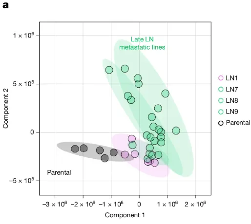
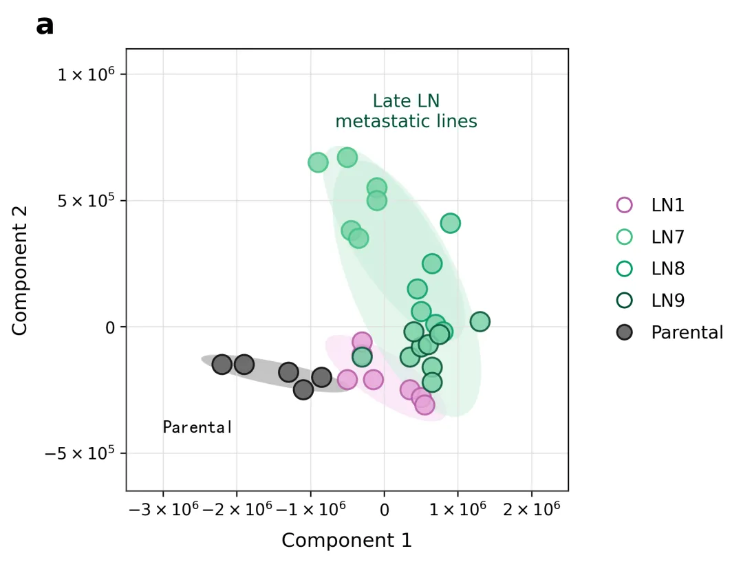
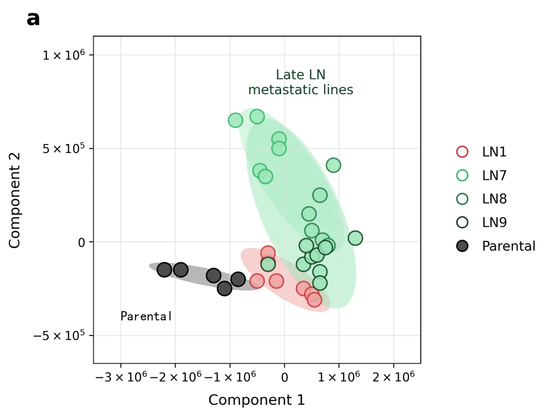
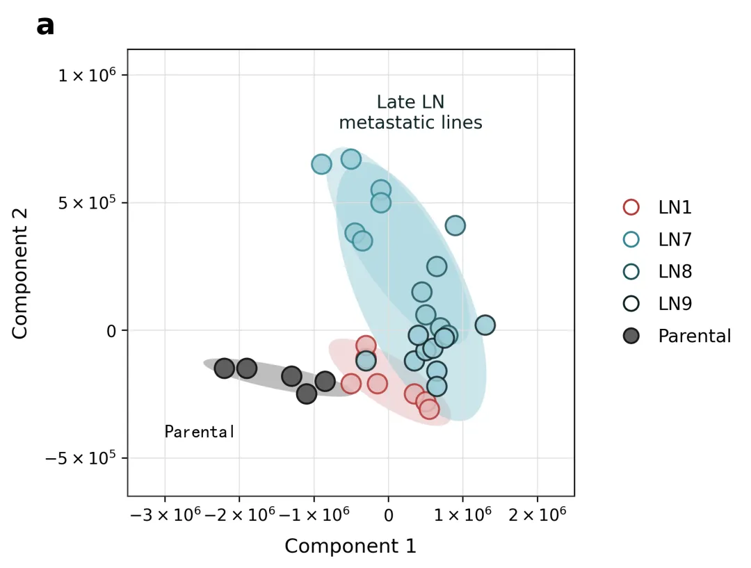
import osimport numpy as npimport pandas as pdimport matplotlib.pyplot as pltimport matplotlib.transforms as transformsfrom matplotlib.patches import Ellipsefrom matplotlib.ticker import FixedLocator# ==========================================# 1. 自动化目录与数据读取检查# ==========================================output_dir = "图表"if not os.path.exists(output_dir):    os.makedirs(output_dir)excel_path = "data.xlsx"if not os.path.exists(excel_path):    raise FileNotFoundError(f"未在当前目录下找到 '{excel_path}' 文件，请先创建并填充数据。")df = pd.read_excel(excel_path)# ==========================================# 2. 置信椭圆绘制辅助函数# ==========================================def draw_confidence_ellipse(ax, x, y, edgecolor, facecolor, alpha=0.15, n_std=2.0):    if len(x) < 3:        return    cov = np.cov(x, y)    pearson = cov[0, 1] / np.sqrt(cov[0, 0] * cov[1, 1])    ell_radius_x = np.sqrt(1 + pearson)    ell_radius_y = np.sqrt(1 - pearson)    ellipse = Ellipse((0, 0), width=ell_radius_x * 2, height=ell_radius_y * 2,                      facecolor=facecolor, edgecolor=edgecolor, alpha=alpha, linewidth=1)    scale_x = np.sqrt(cov[0, 0]) * n_std    mean_x = np.mean(x)    scale_y = np.sqrt(cov[1, 1]) * n_std    mean_y = np.mean(y)    transf = transforms.Affine2D() \        .rotate_deg(45) \        .scale(scale_x, scale_y) \        .translate(mean_x, mean_y)    ellipse.set_transform(transf + ax.transData)    ax.add_patch(ellipse)# ==========================================# 3. 10种专业科研配色方案字典 (符合主流期刊标准)# ==========================================# 每种方案包含两部分：# 'fill': 对应 ['Parental', 'LN1', 'LN7', 'LN8', 'LN9'] 的数据点填充颜色# 'edge': 对应 ['Parental', 'LN1', 'LN7', 'LN8', 'LN9'] 的图例边框及线条颜色color_schemes = {    1: { # 经典 Nature/Science 风格：高对比度清爽自然色系        'fill': ['#6d6d6d', '#e6a3d8', '#79d2a6', '#79d2a6', '#79d2a6'],        'edge': ['#1a1a1a', '#b359a3', '#40bf80', '#009966', '#004d33']    }}# 选择方案 1selected_scheme = color_schemes[3]groups = ['Parental', 'LN1', 'LN7', 'LN8', 'LN9']color_map = dict(zip(groups, selected_scheme['fill']))edge_map = dict(zip(groups, selected_scheme['edge']))fig, ax = plt.subplots(figsize=(6.5, 6.5), dpi=200)ax.set_facecolor('white')ax.grid(True, color='#e0e0e0', linestyle='-', linewidth=0.6, zorder=0)# ==========================================# 4. 核心绘制逻辑# ==========================================# 4.1 绘制置信阴影圈df_p = df[df['Group'] == 'Parental']draw_confidence_ellipse(ax, df_p['Component 1'], df_p['Component 2'],                        edgecolor='none', facecolor=color_map['Parental'], alpha=0.4, n_std=1.8)df_ln1 = df[df['Group'] == 'LN1']draw_confidence_ellipse(ax, df_ln1['Component 1'], df_ln1['Component 2'],                        edgecolor='none', facecolor='#f7d3f2' if selected_scheme == color_schemes[1] else color_map['LN1'], alpha=0.5, n_std=1.9)df_late = df[df['Group'].isin(['LN7', 'LN8', 'LN9'])]draw_confidence_ellipse(ax, df_late['Component 1'], df_late['Component 2'],                        edgecolor='none', facecolor='#cceedd' if selected_scheme == color_schemes[1] else color_map['LN7'], alpha=0.5, n_std=1.8)df_late_sub = df[df['Group'].isin(['LN7', 'LN8'])]draw_confidence_ellipse(ax, df_late_sub['Component 1'], df_late_sub['Component 2'],                        edgecolor='none', facecolor='#bfe8d3' if selected_scheme == color_schemes[1] else color_map['LN8'], alpha=0.4, n_std=1.6)# 4.2 绘制数据散点与图例groups_order = ['LN1', 'LN7', 'LN8', 'LN9', 'Parental']legend_elements = []for grp in groups_order:    grp_data = df[df['Group'] == grp]    color = color_map[grp]    edge_c = edge_map[grp]    if grp == 'Parental':        sc = ax.scatter(grp_data['Component 1'], grp_data['Component 2'],                        color=color, edgecolor=edge_c, s=140, linewidths=1.2, zorder=4)        leg_handle = plt.Line2D([0], [0], marker='o', color='none',                                markerfacecolor=color, markeredgecolor=edge_c,                                markersize=9, markeredgewidth=1.2)    else:        sc = ax.scatter(grp_data['Component 1'], grp_data['Component 2'],                        color=color, edgecolor=edge_c, s=140, linewidths=1.2, alpha=0.85, zorder=5)        leg_handle = plt.Line2D([0], [0], marker='o', color='none',                                markerfacecolor='none', markeredgecolor=edge_c,                                markersize=9, markeredgewidth=1.2)    legend_elements.append((leg_handle, grp))# ==========================================# 5. 坐标轴、标签与文本还原# ==========================================x_ticks = [-3e6, -2e6, -1e6, 0, 1e6, 2e6]y_ticks = [-5e5, 0, 5e5, 1e6]ax.set_xlim(-3.5e6, 2.5e6)ax.set_ylim(-6.5e05, 1.1e6)ax.set_box_aspect(1)ax.xaxis.set_major_locator(FixedLocator(x_ticks))ax.yaxis.set_major_locator(FixedLocator(y_ticks))ax.set_xticklabels(    ['$-3 \\times 10^6$', '$-2 \\times 10^6$', '$-1 \\times 10^6$', '$0$', '$1 \\times 10^6$', '$2 \\times 10^6$'])ax.set_yticklabels(['$-5 \\times 10^5$', '$0$', '$5 \\times 10^5$', '$1 \\times 10^6$'])ax.set_xlabel('Component 1', fontsize=12, labelpad=8)ax.set_ylabel('Component 2', fontsize=12, labelpad=8)ax.spines['top'].set_visible(True)ax.spines['right'].set_visible(True)ax.spines['left'].set_color('#333333')ax.spines['bottom'].set_color('#333333')ax.text(-3.0e6, -4.2e5, 'Parental', fontsize=11, color='black',        fontproperties='SimHei' if os.name == 'nt' else 'sans-serif')ax.text(0.3e6, 8.5e5, 'Late LN\nmetastatic lines', fontsize=11, color=edge_map['LN9'], ha='center', va='center')handles, labels = zip(*legend_elements)ax.legend(handles, labels, loc='center left', bbox_to_anchor=(1.05, 0.5),          frameon=False, handletextpad=0.5, labelspacing=0.8, fontsize=11)plt.tight_layout()fig.canvas.draw()pos = ax.get_position()fig.text(pos.x0 - 0.12, pos.y1 + 0.02, 'a', fontsize=18, fontweight='bold', zorder=10)# ==========================================# 6. 保存输出# ==========================================output_path = os.path.join(output_dir, "PCA_Component_Plot.png")plt.savefig(output_path, bbox_inches='tight', dpi=300)plt.close()print(f"\n图像已成功保存至: {output_path}")