Python 从散斑图中提取位移场和应变云图(含代码)

引言

试样变形过程通常需要通过照片、视频或高速相机图像进行记录。然而如果只是把加载前后的照片放在论文或报告中，能够展示试样外观变化，却很难进一步说明变形的方向、位移的大小以及局部变形集中区域。对于很多试验结果来说，真正有价值的信息并不只是“试样变形了”，而是“哪里变形最大”“变形主要沿什么方向发展”“局部应变是否已经开始集中”。数字图像相关方法，也就是 DIC，正是围绕这一问题展开的。它的基本思想是：在加载前图像中选取局部窗口，在加载后图像中寻找最相似的位置，由此得到该区域的位移；当多个局部窗口都完成匹配后，就可以得到试样表面的位移场，并进一步由位移梯度计算应变场。本文用Python构造一组模拟散斑试样图，生成加载前后图像，并通过简化版图像匹配方法提取位移矢量场和等效应变云图。这个例子并不是替代专业 DIC 软件，而是用来展示 DIC 后处理的基本思路：一张普通散斑图如何从“图像”转化为“位移场”，再进一步转化为论文中常见的“应变云图”。

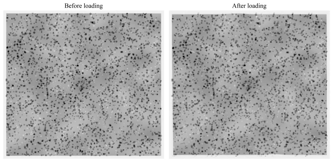
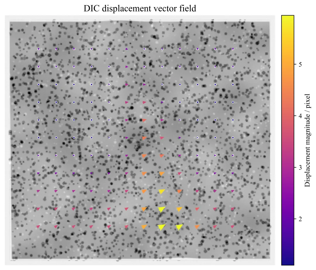
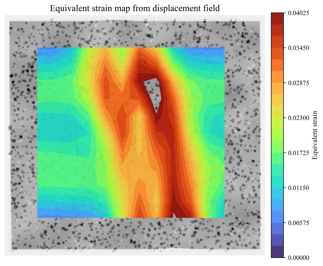
import osimport numpy as npimport matplotlibmatplotlib.use("Agg")import matplotlib.pyplot as pltfrom scipy.ndimage import gaussian_filter, map_coordinatesnp.random.seed(2026)plt.rcParams["font.family"] = "Times New Roman"plt.rcParams["axes.unicode_minus"] = Falseplt.rcParams["figure.dpi"] = 160plt.rcParams["savefig.dpi"] = 500out_dir = "simple_dic_results_noborder"os.makedirs(out_dir, exist_ok=True)H, W = 620, 820# 试样区域x_left, x_right = 160, 660y_top, y_bottom = 80, 540Y, X = np.mgrid[0:H, 0:W]specimen_mask = (    (X >= x_left) &    (X <= x_right) &    (Y >= y_top) &    (Y <= y_bottom))def set_specimen_view(ax, pad=10):    """    只显示试样附近区域，去掉外围大块背景。    """    ax.set_xlim(x_left - pad, x_right + pad)    ax.set_ylim(y_bottom + pad, y_top - pad)    ax.axis("off")def draw_random_speckles(img, mask, n_dark=2800, n_light=900):    """    在试样区域内生成随机散斑。    """    ys, xs = np.where(mask)    # 暗色散斑    for _ in range(n_dark):        k = np.random.randint(0, len(xs))        cx = xs[k]        cy = ys[k]        r = np.random.uniform(1.2, 3.2)        x0 = max(0, int(cx - 4))        x1 = min(W, int(cx + 5))        y0 = max(0, int(cy - 4))        y1 = min(H, int(cy + 5))        yy, xx = np.mgrid[y0:y1, x0:x1]        disk = (xx - cx) ** 2 + (yy - cy) ** 2 <= r ** 2        img[y0:y1, x0:x1][disk] -= np.random.uniform(0.18, 0.34)    # 亮色散斑    for _ in range(n_light):        k = np.random.randint(0, len(xs))        cx = xs[k]        cy = ys[k]        r = np.random.uniform(1.0, 2.4)        x0 = max(0, int(cx - 4))        x1 = min(W, int(cx + 5))        y0 = max(0, int(cy - 4))        y1 = min(H, int(cy + 5))        yy, xx = np.mgrid[y0:y1, x0:x1]        disk = (xx - cx) ** 2 + (yy - cy) ** 2 <= r ** 2        img[y0:y1, x0:x1][disk] += np.random.uniform(0.06, 0.14)    return imgdef normalized_correlation(a, b):    """    归一化相关系数。    """    aa = a - a.mean()    bb = b - b.mean()    denom = np.sqrt(np.sum(aa ** 2) * np.sum(bb ** 2)) + 1e-12    return np.sum(aa * bb) / denom#生成加载前散斑试样图# 背景（保留但绘图时会裁掉大部分）img_before = np.ones((H, W)) * 0.94img_before += np.random.normal(0, 0.006, size=(H, W))# 试样基底：低频灰度纹理low_freq_noise = gaussian_filter(np.random.normal(0, 1, size=(H, W)), sigma=18)low_freq_noise = (low_freq_noise - low_freq_noise.mean()) / (low_freq_noise.std() + 1e-8)specimen_base = 0.66 + 0.035 * low_freq_noiseimg_before[specimen_mask] = specimen_base[specimen_mask]# 添加散斑img_before = draw_random_speckles(img_before, specimen_mask)# 轻微模糊，模拟相机成像img_before = gaussian_filter(img_before, sigma=0.55)# 不再人为添加试样边框img_before = np.clip(img_before, 0, 1)# 构造加载后的真实位移场，并生成加载后图像xn = (X - x_left) / (x_right - x_left)yn = (Y - y_top) / (y_bottom - y_top)# 基本压缩 + 剪切u_true = 1.5 + 5.0 * (yn - 0.5)v_true = -5.5 * (yn - 0.5)# 局部剪切带，模拟局部变形集中band_center = x_left + (x_right - x_left) * (0.42 + 0.24 * yn)band_width = 32.0shear_band = np.exp(-((X - band_center) / band_width) ** 2)u_true += 4.2 * shear_bandv_true += -2.3 * shear_band# 试样外不发生变形u_true = u_true * specimen_maskv_true = v_true * specimen_mask# 反向映射生成加载后图像coords_y = Y - v_truecoords_x = X - u_trueimg_after = map_coordinates(    img_before,    [coords_y, coords_x],    order=1,    mode="reflect")# 加入轻微拍摄噪声和亮度变化img_after += np.random.normal(0, 0.006, size=(H, W))img_after = 0.985 * img_after + 0.008img_after = np.clip(img_after, 0, 1)# 局部窗口匹配提取位移subset_size = 31half = subset_size // 2search_radius = 10grid_step = 34grid_x = np.arange(x_left + 55, x_right - 55, grid_step)grid_y = np.arange(y_top + 55, y_bottom - 55, grid_step)GX, GY = np.meshgrid(grid_x, grid_y)U = np.zeros_like(GX, dtype=float)V = np.zeros_like(GY, dtype=float)C = np.zeros_like(GX, dtype=float)for iy in range(GY.shape[0]):    for ix in range(GX.shape[1]):        cx = int(GX[iy, ix])        cy = int(GY[iy, ix])        template = img_before[            cy - half: cy + half + 1,            cx - half: cx + half + 1        ]        best_score = -1e9        best_dx = 0        best_dy = 0        for dy in range(-search_radius, search_radius + 1):            for dx in range(-search_radius, search_radius + 1):                tx = cx + dx                ty = cy + dy                patch = img_after[                    ty - half: ty + half + 1,                    tx - half: tx + half + 1                ]                if patch.shape != template.shape:                    continue                score = normalized_correlation(template, patch)                if score > best_score:                    best_score = score                    best_dx = dx                    best_dy = dy        U[iy, ix] = best_dx        V[iy, ix] = best_dy        C[iy, ix] = best_score# 平滑位移场，减少匹配噪声U_smooth = gaussian_filter(U, sigma=0.7)V_smooth = gaussian_filter(V, sigma=0.7)disp_mag = np.sqrt(U_smooth ** 2 + V_smooth ** 2)# 由位移场计算应变场dU_dy, dU_dx = np.gradient(U_smooth, grid_step, grid_step)dV_dy, dV_dx = np.gradient(V_smooth, grid_step, grid_step)exx = dU_dxeyy = dV_dygamma_xy = dU_dy + dV_dxequiv_strain = np.sqrt(exx ** 2 + eyy ** 2 + 0.5 * gamma_xy ** 2)equiv_strain = gaussian_filter(equiv_strain, sigma=0.6)# 加载前后散斑图fig, axes = plt.subplots(1, 2, figsize=(10.2, 5.6))axes[0].imshow(img_before, cmap="gray", vmin=0, vmax=1)axes[0].set_title("Before loading", fontsize=14)set_specimen_view(axes[0], pad=10)axes[1].imshow(img_after, cmap="gray", vmin=0, vmax=1)axes[1].set_title("After loading", fontsize=14)set_specimen_view(axes[1], pad=10)plt.tight_layout()fig1_path = os.path.join(out_dir, "fig1_speckle_before_after.png")plt.savefig(fig1_path, bbox_inches="tight", facecolor="white")plt.close(fig)# 位移矢量场fig, ax = plt.subplots(figsize=(7.1, 6.5))# 背景变浅，避免遮挡箭头ax.imshow(img_after, cmap="gray", vmin=0, vmax=1)# 先画白色粗箭头作为底ax.quiver(    GX,    GY,    U_smooth,    V_smooth,    color="white",    angles="xy",    scale_units="xy",    scale=0.45,    width=0.009,    headwidth=4.2,    headlength=5.2,    alpha=0.90,    pivot="mid")# 再画彩色箭头q = ax.quiver(    GX,    GY,    U_smooth,    V_smooth,    disp_mag,    cmap="plasma",    angles="xy",    scale_units="xy",    scale=0.45,    width=0.0055,    headwidth=4.2,    headlength=5.2,    alpha=0.98,    pivot="mid")# 控制色带范围，提升整体对比度q.set_clim(    np.percentile(disp_mag, 5),    np.percentile(disp_mag, 98))ax.set_title("DIC displacement vector field", fontsize=14)set_specimen_view(ax, pad=10)cbar = fig.colorbar(q, ax=ax, shrink=0.84, pad=0.02)cbar.set_label("Displacement magnitude / pixel", fontsize=11)plt.tight_layout()fig2_path = os.path.join(out_dir, "fig2_displacement_vector_field.png")plt.savefig(fig2_path, bbox_inches="tight", facecolor="white")plt.close(fig)# 等效应变云图fig, ax = plt.subplots(figsize=(7.1, 6.5))# 轻背景，仅作为辅助ax.imshow(img_after, cmap="gray", vmin=0, vmax=1)vmax = np.percentile(equiv_strain, 98)levels = np.linspace(0, vmax, 22)cf = ax.contourf(    GX,    GY,    equiv_strain,    levels=levels,    cmap="turbo",    alpha=0.90)ax.set_title("Equivalent strain map from displacement field", fontsize=14)set_specimen_view(ax, pad=10)cbar = fig.colorbar(cf, ax=ax, shrink=0.84, pad=0.02)cbar.set_label("Equivalent strain", fontsize=11)plt.tight_layout()fig3_path = os.path.join(out_dir, "fig3_equivalent_strain_map.png")plt.savefig(fig3_path, bbox_inches="tight", facecolor="white")plt.close(fig)

特别声明：

以上代码与文案均为网上资料整合而成，仅供广大同行们参考学习，如有侵权请联系删除。