先看图:
简单地总结下上面的六张图
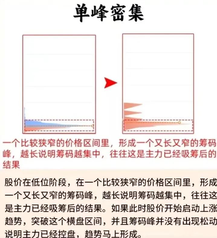
1. 单峰密集 - 主力吸筹完成,高度控盘
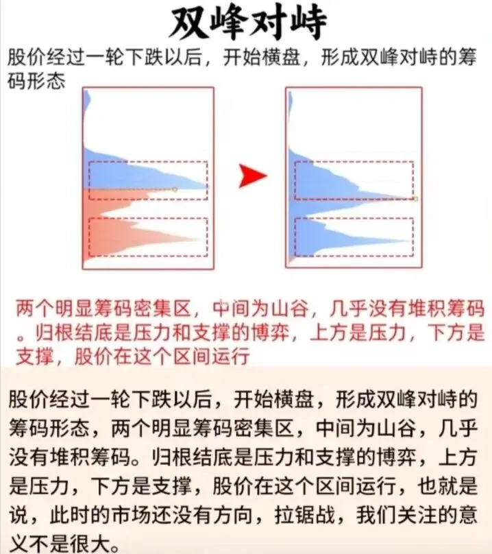
2. 双峰对峙 - 压力和支撑博弈,方向不明
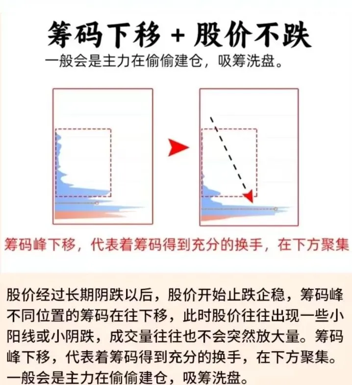
3. 筹码下移+股价不跌 - 主力偷偷建仓
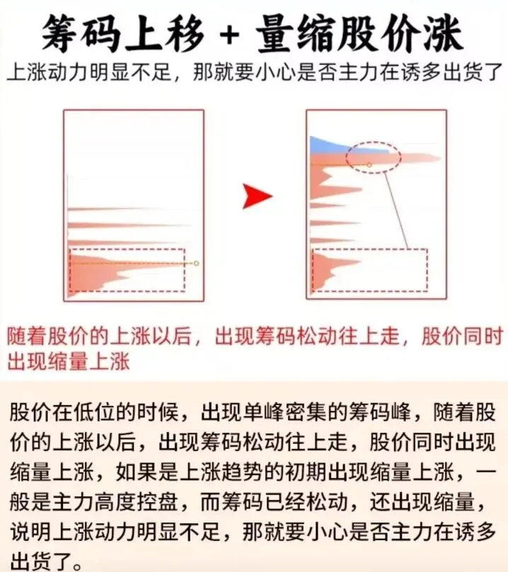
4. 筹码上移+量缩股价涨 - 可能诱多出货
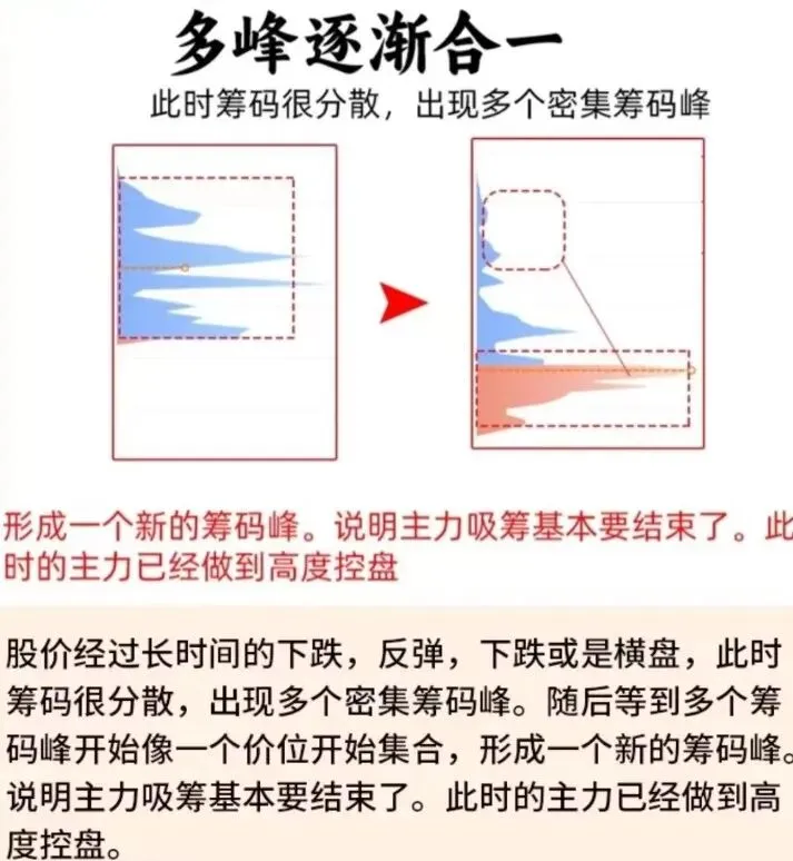
5. 多峰逐渐合一 - 主力高度控盘,吸筹结束
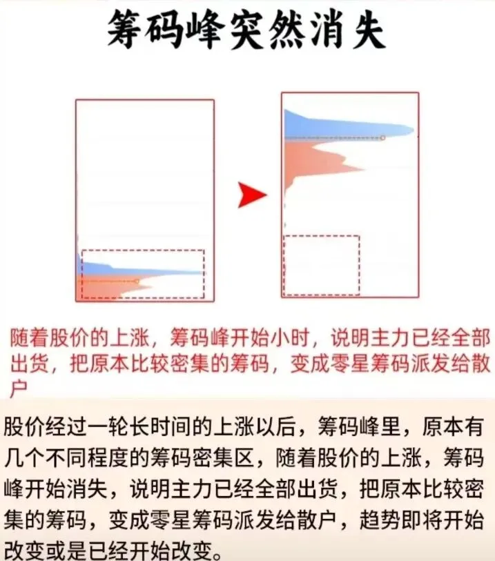
6. 筹码峰突然消失 - 主力出货完成。
那么根据筹码峰指标进行选股,是一个非常常用且有效的方法。但仅仅靠人工去从五千多只股票中去逐一分析,等分析完,黄花菜都凉了!那么,只有依靠电脑去做这件事,才能高效、准确地去完成。
下面就是根据上述逻辑,使用python代码写出的选股方案,仅供参考:
import pandas as pd
import numpy as np
import talib
class ChipPeakSelector:
"""
筹码峰形态选股模型
注:实际筹码分布数据需要专门的筹码分布计算,这里用价格和成交量近似模拟
"""
def __init__(self, df, price_col='close', volume_col='volume'):
"""
初始化
:param df: 包含OHLCV数据的DataFrame
:param price_col: 价格列名
:param volume_col: 成交量列名
"""
self.df = df.copy()
self.price_col = price_col
self.volume_col = volume_col
def calculate_price_distribution(self, window=20):
"""
模拟价格分布(简化版筹码计算)
实际应用中应使用专门的筹码分布算法
"""
df = self.df
# 计算价格区间
df['price_range'] = (df['high'] - df['low']) / df['low'] * 100
# 计算移动平均和标准差,用于判断密集区
df['ma'] = df[self.price_col].rolling(window=window).mean()
df['std'] = df[self.price_col].rolling(window=window).std()
# 价格密集度指标(简化)
df['price_density'] = df['std'] / df['ma']
return df
# ========== 形态识别函数 ==========
def detect_single_peak(self, window=30, density_threshold=0.05):
"""
识别单峰密集形态
:param window: 观察窗口
:param density_threshold: 价格密集度阈值
"""
df = self.calculate_price_distribution(window)
# 单峰密集特征:
# 1. 价格波动小(低标准差)
# 2. 成交量相对稳定
# 3. 价格在窄幅区间运行
# 计算价格波动率
df['volatility'] = df[self.price_col].pct_change().rolling(window).std()
# 计算成交量稳定性
df['volume_ma'] = df[self.volume_col].rolling(window).mean()
df['volume_std'] = df[self.volume_col].rolling(window).std()
df['volume_stability'] = df['volume_std'] / df['volume_ma']
# 识别条件
condition = (
(df['price_density'] < density_threshold) & # 价格密集
(df['volatility'] < df['volatility'].quantile(0.3)) & # 低波动
(df['volume_stability'] < 0.5) # 成交量相对稳定
)
return condition
def detect_double_peak(self, window=60):
"""
识别双峰对峙形态
"""
df = self.df
# 双峰特征:
# 1. 价格在一定区间内震荡
# 2. 可能存在两个价格密集区
# 计算布林带,观察价格是否在通道内运行
df['bb_upper'], df['bb_middle'], df['bb_lower'] = talib.BBANDS(
df[self.price_col], timeperiod=20, nbdevup=2, nbdevdn=2
)
# 价格在布林带中轨附近震荡的比例
df['bb_position'] = (df[self.price_col] - df['bb_lower']) / (df['bb_upper'] - df['bb_lower'])
# 震荡指标
df['atr'] = talib.ATR(df['high'], df['low'], df['close'], timeperiod=14)
df['atr_ratio'] = df['atr'] / df[self.price_col]
# 识别条件:价格在中轨附近震荡,波动率适中
condition = (
(df['bb_position'] > 0.3) & (df['bb_position'] < 0.7) &
(df['atr_ratio'] > df['atr_ratio'].quantile(0.3)) &
(df['atr_ratio'] < df['atr_ratio'].quantile(0.7))
)
return condition
def detect_chip_down_no_price_down(self, window=30):
"""
识别筹码下移但股价不跌(主力吸筹)
"""
df = self.df
# 特征:
# 1. 价格相对稳定或小幅上涨
# 2. 成交量温和放大
# 3. 波动率可能降低
# 价格趋势
df['price_ma_short'] = df[self.price_col].rolling(10).mean()
df['price_ma_long'] = df[self.price_col].rolling(30).mean()
# 成交量趋势
df['volume_ma_short'] = df[self.volume_col].rolling(10).mean()
df['volume_ma_long'] = df[self.volume_col].rolling(30).mean()
# 识别条件
condition = (
(df['price_ma_short'] > df['price_ma_long']) & # 短期趋势向上
(df['volume_ma_short'] > df['volume_ma_long'] * 0.8) & # 成交量温和
(df['volume_ma_short'] < df['volume_ma_long'] * 1.5) # 不放巨量
)
return condition
def detect_chip_up_volume_down(self):
"""
识别筹码上移但量缩股价涨(可能诱多出货)
"""
df = self.df
# 特征:
# 1. 价格上涨但成交量萎缩
# 2. 可能创出新高但量价背离
# 价格创新高
df['price_new_high'] = df[self.price_col] > df[self.price_col].rolling(20).max().shift(1)
# 成交量萎缩
df['volume_ma5'] = df[self.volume_col].rolling(5).mean()
df['volume_ma20'] = df[self.volume_col].rolling(20).mean()
df['volume_decline'] = df['volume_ma5'] < df['volume_ma20']
# 价格与成交量背离
price_change = df[self.price_col].pct_change(5)
volume_change = df[self.volume_col].pct_change(5)
df['price_volume_divergence'] = (price_change > 0) & (volume_change < 0)
condition = (
df['price_new_high'] &
df['volume_decline'] &
df['price_volume_divergence']
)
return condition
def detect_multi_peak_convergence(self, window=60):
"""
识别多峰逐渐合一(主力高度控盘)
"""
df = self.calculate_price_distribution(window)
# 多峰合一特征:
# 1. 价格波动率逐渐降低
# 2. 价格区间收窄
# 3. 成交量可能萎缩
# 波动率变化趋势
df['volatility_short'] = df[self.price_col].pct_change().rolling(10).std()
df['volatility_long'] = df[self.price_col].pct_change().rolling(30).std()
df['volatility_decreasing'] = df['volatility_short'] < df['volatility_long']
# 价格区间收窄
df['range_short'] = (df['high'].rolling(10).max() - df['low'].rolling(10).min()) / df['low'].rolling(10).min()
df['range_long'] = (df['high'].rolling(30).max() - df['low'].rolling(30).min()) / df['low'].rolling(30).min()
df['range_narrowing'] = df['range_short'] < df['range_long']
condition = (
df['volatility_decreasing'] &
df['range_narrowing'] &
(df['price_density'] < df['price_density'].quantile(0.3))
)
return condition
# ========== 综合选股函数 ==========
def select_stocks_by_pattern(self, pattern_name):
"""
根据指定形态选股
:param pattern_name: 形态名称
"""
pattern_functions = {
'single_peak': self.detect_single_peak,
'double_peak': self.detect_double_peak,
'chip_down_no_price_down': self.detect_chip_down_no_price_down,
'chip_up_volume_down': self.detect_chip_up_volume_down,
'multi_peak_convergence': self.detect_multi_peak_convergence
}
if pattern_name not in pattern_functions:
raise ValueError(f"未知形态: {pattern_name}")
signal = pattern_functions[pattern_name]()
return signal
def generate_signals(self):
"""
生成所有形态的信号
"""
signals = pd.DataFrame(index=self.df.index)
# 检测各种形态
signals['single_peak'] = self.detect_single_peak()
signals['double_peak'] = self.detect_double_peak()
signals['chip_down_no_price_down'] = self.detect_chip_down_no_price_down()
signals['chip_up_volume_down'] = self.detect_chip_up_volume_down()
signals['multi_peak_convergence'] = self.detect_multi_peak_convergence()
# 筹码峰消失的判断(需要更长周期观察)
signals['chip_disappear'] = self.detect_chip_disappear()
return signals
def detect_chip_disappear(self, window=50):
"""
识别筹码峰消失(主力出货)
"""
df = self.df
# 特征:
# 1. 价格大幅上涨后
# 2. 成交量异常放大后萎缩
# 3. 价格开始下跌或横盘
# 价格涨幅
df['price_increase'] = df[self.price_col] / df[self.price_col].rolling(window).min() - 1
# 成交量异常
df['volume_ratio'] = df[self.volume_col] / df[self.volume_col].rolling(20).mean()
df['volume_spike'] = df['volume_ratio'] > 2
# 价格转折
df['price_ma20'] = df[self.price_col].rolling(20).mean()
df['price_below_ma'] = df[self.price_col] < df['price_ma20']
condition = (
(df['price_increase'] > 0.5) & # 涨幅超过50%
df['price_below_ma'] & # 价格跌破均线
(df['volume_ratio'] < 0.8) # 成交量萎缩
)
return condition
# ========== 使用示例 ==========
if __name__ == "__main__":
# 示例:加载股票数据
# df = pd.read_csv('stock_data.csv', index_col='date', parse_dates=True)
# 创建示例数据
dates = pd.date_range('2023-01-01', periods=200, freq='D')
np.random.seed(42)
example_data = pd.DataFrame({
'open': np.random.randn(200).cumsum() + 100,
'high': np.random.randn(200).cumsum() + 102,
'low': np.random.randn(200).cumsum() + 98,
'close': np.random.randn(200).cumsum() + 100,
'volume': np.random.randint(100000, 1000000, 200)
}, index=dates)
# 确保价格合理
example_data['high'] = example_data[['open', 'close']].max(axis=1) + np.abs(np.random.randn(200))
example_data['low'] = example_data[['open', 'close']].min(axis=1) - np.abs(np.random.randn(200))
# 创建选股器实例
selector = ChipPeakSelector(example_data)
# 检测单峰密集形态
single_peak_signals = selector.detect_single_peak()
print(f"单峰密集信号数量: {single_peak_signals.sum()}")
# 检测多峰合一形态
convergence_signals = selector.detect_multi_peak_convergence()
print(f"多峰合一信号数量: {convergence_signals.sum()}")
# 获取所有信号
all_signals = selector.generate_signals()
print("\n各形态信号统计:")
print(all_signals.sum())
# 寻找符合条件的股票
# 例如:寻找出现单峰密集且筹码下移的股票
target_signals = all_signals['single_peak'] & all_signals['chip_down_no_price_down']
print(f"\n目标形态(单峰密集+筹码下移)出现次数: {target_signals.sum()}")
使用建议:
1. 数据要求:
· 需要OHLCV(开盘、最高、最低、收盘、成交量)数据
· 建议使用日线或更长周期的数据
· 至少需要60个交易日的连续数据
2. 参数优化:
· 可根据不同股票特性调整阈值参数
· 窗口期可根据投资周期调整(短线用较小窗口,长线用较大窗口)
3. 注意事项:
· 这是简化版的筹码模型,实际筹码分布需要专门的算法
· 应结合其他技术指标(如MACD、RSI等)和基本面分析
· 回测验证策略有效性非常重要
4. 风险提示:
· 任何技术指标都有滞后性
· 股市有风险,投资需谨慎
· 建议在实际交易前进行充分的回测和验证
这个模型提供了基本的框架,你可以根据实际需求进行调整和扩展。可以私信交流,共赢未来。