引言
在深度学习推理领域,CUDA编程技术的掌握已成为工程师提升模型性能的关键技能。随着模型规模不断扩大和实时性要求日益严格,如何充分利用GPU的并行计算能力成为技术挑战。本文将从CUDA架构原理出发,深入探讨推理优化的核心技术路径,分享实用的编程技巧和实战经验,帮助读者构建高效的深度学习推理系统。一、CUDA架构与并行计算基础
1.1 GPU硬件架构演进
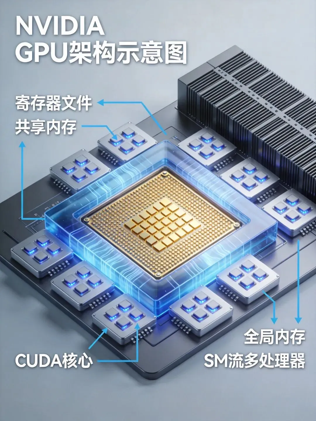
现代NVIDIA GPU基于SIMT(Single Instruction Multiple Threads)架构,通过大规模并行线程实现高性能计算。以RTX 4090为例,其包含16384个CUDA核心,分为多个SM(Streaming Multiprocessor),每个SM具备独立的共享内存、寄存器文件和调度单元。图1: NVIDIA GPU硬件架构层次化布局示意图// 获取GPU设备信息示例cudaDeviceProp prop;cudaGetDeviceProperties(&prop, 0);printf("GPU: %s\n", prop.name);printf("SM数量: %d\n", prop.multiProcessorCount);printf("每SM的CUDA核心数: %d\n", prop.maxThreadsPerMultiProcessor);printf("全局内存: %.2f GB\n", prop.totalGlobalMem / (1024.0 * 1024.0 * 1024.0));
1.2 线程层次与内存模型
- 线程(Thread)
- 线程块(Block)
- 线程网格(Grid)
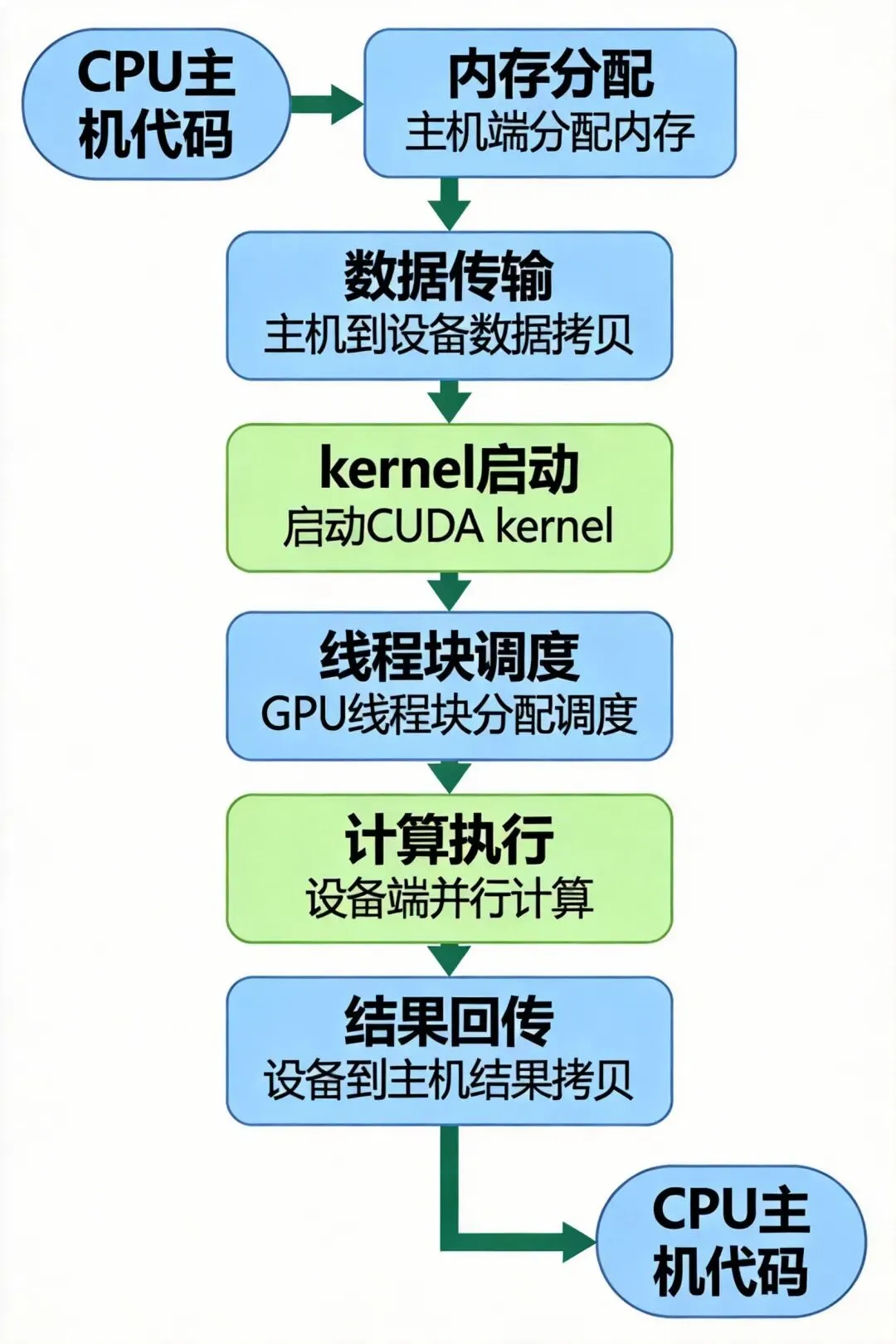
图2: CUDA kernel从CPU到GPU的完整执行流程__global__ voidmatrixMulKernel(float* A, float* B, float* C, int width) { // 使用共享内存优化矩阵乘法 __shared__ float ds_A[TILE_SIZE][TILE_SIZE]; __shared__ float ds_B[TILE_SIZE][TILE_SIZE]; int bx = blockIdx.x; int by = blockIdx.y; int tx = threadIdx.x; int ty = threadIdx.y; // 计算全局索引 int row = by * TILE_SIZE + ty; int col = bx * TILE_SIZE + tx; float sum = 0.0f; // 分块计算 for (int i = 0; i < (width + TILE_SIZE - 1) / TILE_SIZE; ++i) { // 加载数据到共享内存 if (row < width && i * TILE_SIZE + tx < width) ds_A[ty][tx] = A[row * width + i * TILE_SIZE + tx]; else ds_A[ty][tx] = 0.0f; if (i * TILE_SIZE + ty < width && col < width) ds_B[ty][tx] = B[(i * TILE_SIZE + ty) * width + col]; else ds_B[ty][tx] = 0.0f; __syncthreads(); // 同步确保数据加载完成 // 计算部分乘积 for (int k = 0; k < TILE_SIZE; ++k) sum += ds_A[ty][k] * ds_B[k][tx]; __syncthreads(); // 同步确保计算完成 } // 写入结果 if (row < width && col < width) C[row * width + col] = sum;}
二、深度学习推理优化核心策略
2.1 内存访问优化
内存合并访问是提升性能的关键。相邻线程应访问连续的内存地址,充分利用内存带宽。// 优化前: 非合并访问__global__ voidbad_access(float* data) { int idx = threadIdx.x + blockIdx.x * blockDim.x; // 跨步访问,导致内存访问效率低下 data[idx * 4] *= 2.0f; }// 优化后: 合并访问__global__ voidgood_access(float* data) { int idx = threadIdx.x + blockIdx.x * blockDim.x; // 连续访问,充分利用内存带宽 data[idx] *= 2.0f;}
对于频繁访问的数据,使用共享内存可显著减少全局内存访问延迟。__global__ void convolution_shared(float* input, float* filter, float* output, int width, int height, int filter_size) { extern __shared__ float shared_data[]; int tx = threadIdx.x; int ty = threadIdx.y; int bx = blockIdx.x; int by = blockIdx.y; // 计算输出位置 int output_x = bx * blockDim.x + tx; int output_y = by * blockDim.y + ty; // 加载输入数据到共享内存(包含halo区域) int halo = filter_size / 2; int load_x = bx * blockDim.x + tx - halo; int load_y = by * blockDim.y + ty - halo; // 边界检查 if (load_x >= 0 && load_x < width && load_y >= 0 && load_y < height) { shared_data[ty * (blockDim.x + 2 * halo) + tx] = input[load_y * width + load_x]; } else { shared_data[ty * (blockDim.x + 2 * halo) + tx] = 0.0f; } __syncthreads(); // 执行卷积计算 if (output_x < width - filter_size + 1 && output_y < height - filter_size + 1) { float sum = 0.0f; for (int fy = 0; fy < filter_size; fy++) { for (int fx = 0; fx < filter_size; fx++) { int local_x = tx + fx; int local_y = ty + fy; sum += shared_data[local_y * (blockDim.x + 2 * halo) + local_x] * filter[fy * filter_size + fx]; } } output[output_y * (width - filter_size + 1) + output_x] = sum; }}
2.2 计算优化技术
// 使用WMMA API进行Tensor Core计算#include<mma.h>using namespace nvcuda::wmma;__global__ voidtensor_core_gemm(half* a, half* b, float* c, int M, int N, int K) { // 初始化fragment wmma::fragment<matrix_a, 16, 16, 16, half, row_major> a_frag; wmma::fragment<matrix_b, 16, 16, 16, half, col_major> b_frag; wmma::fragment<accumulator, 16, 16, 16, float> c_frag; // 加载矩阵片段 wmma::load_matrix_sync(a_frag, a, K); wmma::load_matrix_sync(b_frag, b, K); // 矩阵乘累加 wmma::mma_sync(c_frag, a_frag, b_frag, c_frag); // 存储结果 wmma::store_matrix_sync(c, c_frag, N, mem_row_major);}
通过增加指令级并行度,隐藏延迟,提升计算资源利用率。__global__ voidilp_optimized_kernel(float* data, int size) { int idx = threadIdx.x + blockIdx.x * blockDim.x * 4; int stride = blockDim.x * gridDim.x; // 展开4次循环,增加指令级并行 for (int i = idx; i < size; i += stride * 4) { float v0 = data[i]; float v1 = data[i + stride]; float v2 = data[i + stride * 2]; float v3 = data[i + stride * 3]; // 独立计算,减少依赖 data[i] = sqrtf(v0) + 1.0f; data[i + stride] = sqrtf(v1) + 2.0f; data[i + stride * 2] = sqrtf(v2) + 3.0f; data[i + stride * 3] = sqrtf(v3) + 4.0f; }}
三、高级优化技巧与工程实践
3.1 流(Stream)并发执行
利用CUDA流实现计算与数据传输的重叠,提升整体吞吐量。class MultiStreamExecutor {public: MultiStreamExecutor(int num_streams = 4) : num_streams_(num_streams) { streams_.resize(num_streams_); events_.resize(num_streams_); for (int i = 0; i < num_streams_; ++i) { cudaStreamCreate(&streams_[i]); cudaEventCreate(&events_[i]); } } ~MultiStreamExecutor() { for (int i = 0; i < num_streams_; ++i) { cudaStreamDestroy(streams_[i]); cudaEventDestroy(events_[i]); } } voidexecuteAsync(void* d_in, void* d_out, size_t size, cudaStream_t stream) { // 异步数据传输 cudaMemcpyAsync(d_in, h_in_, size, cudaMemcpyHostToDevice, stream); // 异步计算 dim3 block(256); dim3 grid((size + block.x - 1) / block.x); process_kernel<<<grid, block, 0, stream>>>(d_in, d_out, size); // 异步数据回传 cudaMemcpyAsync(h_out_, d_out, size, cudaMemcpyDeviceToHost, stream); } voidsynchronize(){ for (int i = 0; i < num_streams_; ++i) { cudaStreamSynchronize(streams_[i]); } }private: std::vector<cudaStream_t> streams_; std::vector<cudaEvent_t> events_; int num_streams_; void* h_in_; void* h_out_;};
3.2 图(Graph)优化
CUDA Graph可减少kernel启动开销,特别适用于小batch推理场景。cudaGraph_t createInferenceGraph(){ cudaGraph_t graph; cudaGraphCreate(&graph, 0); // 创建计算节点 cudaGraphNode_t preprocess_node, inference_node, postprocess_node; // 预处理kernel节点 cudaKernelNodeParams preprocess_params = {0}; preprocess_params.func = (void*)preprocess_kernel; preprocess_params.gridDim = dim3(32, 32); preprocess_params.blockDim = dim3(32, 32); cudaGraphAddKernelNode(&preprocess_node, graph, NULL, 0, &preprocess_params); // 推理kernel节点 cudaKernelNodeParams inference_params = {0}; inference_params.func = (void*)inference_kernel; inference_params.gridDim = dim3(64, 64); inference_params.blockDim = dim3(16, 16); cudaGraphAddKernelNode(&inference_node, graph, &preprocess_node, 1, &inference_params); // 后处理kernel节点 cudaKernelNodeParams postprocess_params = {0}; postprocess_params.func = (void*)postprocess_kernel; postprocess_params.gridDim = dim3(32, 32); postprocess_params.blockDim = dim3(32, 32); cudaGraphAddKernelNode(&postprocess_node, graph, &inference_node, 1, &postprocess_params); return graph;}// 执行图推理voidexecuteGraphInference(cudaGraph_t graph, cudaGraphExec_t* exec){ // 实例化图 cudaGraphInstantiate(exec, graph, NULL, NULL, 0); // 启动图执行 cudaGraphLaunch(*exec, 0); cudaStreamSynchronize(0);}
3.3 精度优化策略
通过混合精度计算和量化技术,在保持精度的同时大幅提升推理速度。// FP16推理实现__global__ voidfp16_inference(half* input, half* weight, half* output, int input_size, int output_size) { int idx = blockIdx.x * blockDim.x + threadIdx.x; if (idx >= output_size) return; half sum = 0.0f; for (int i = 0; i < input_size; ++i) { // 使用半精度浮点计算 sum = __hfma(input[i], weight[idx * input_size + i], sum); } output[idx] = sum;}// INT8量化推理__global__ voidint8_inference(int8_t* input, int8_t* weight, int32_t* output, float input_scale, float weight_scale, float output_scale, int input_size, int output_size) { int idx = blockIdx.x * blockDim.x + threadIdx.x; if (idx >= output_size) return; int32_t sum = 0; for (int i = 0; i < input_size; ++i) { // 8位整数累加 sum += input[i] * weight[idx * input_size + i]; } // 反量化到浮点 output[idx] = (int32_t)(sum * input_scale * weight_scale / output_scale);}
四、性能分析与调试工具
4.1 Nsight Systems分析
使用Nsight Systems进行整体性能分析,识别性能瓶颈。# 收集性能数据nsys profile --stats=true --trace=cuda,nvtx \ --output=profile_report ./inference_app# 分析关键指标# - GPU利用率# - 内存传输时间# - Kernel执行时间# - 流并发效率
4.2 Nsight Compute优化
# 详细kernel分析ncu --set full ./inference_app# 关注指标:# - DRAM吞吐量# - L1/Shared Memory命中率# - Warp执行效率# - Occupancy
4.3 自定义性能监控
class PerformanceMonitor {public: voidstart() { cudaEventCreate(&start_); cudaEventCreate(&stop_); cudaEventRecord(start_); } voidstop() { cudaEventRecord(stop_); cudaEventSynchronize(stop_); cudaEventElapsedTime(&elapsed_time_, start_, stop_); } floatgetElapsedTime() const { return elapsed_time_; } voidprintReport(const std::string& kernel_name) { printf("%s: %.3f ms\n", kernel_name.c_str(), elapsed_time_); }private: cudaEvent_t start_, stop_; float elapsed_time_;};// 使用示例PerformanceMonitor monitor;monitor.start();my_kernel<<<grid, block>>>(d_data, size);monitor.stop();monitor.printReport("my_kernel");
五、实战案例:ResNet推理优化
5.1 优化前性能分析
原始ResNet-50推理在RTX 4090上的基准性能:Batch Size 1: 2.3ms/image5.2 优化策略实施
- Kernel Fusion: 将BatchNorm+ReLU融合到Conv层
- Shared Memory Tiling
- Tensor Core加速
- 流水线并行
// 融合Kernel示例__global__ void fused_conv_bn_relu( half* input, half* weight, float* bias, float* bn_mean, float* bn_var, float bn_epsilon, half* output, int height, int width, int in_channels, int out_channels) { // 外部循环 int out_c = blockIdx.z * blockDim.z + threadIdx.z; int out_y = blockIdx.y * blockDim.y + threadIdx.y; int out_x = blockIdx.x * blockDim.x + threadIdx.x; if (out_c >= out_channels || out_y >= height || out_x >= width) return; // 卷积计算 float conv_sum = 0.0f; for (int in_c = 0; in_c < in_channels; ++in_c) { for (int ky = 0; ky < 3; ++ky) { for (int kx = 0; kx < 3; ++kx) { int in_y = out_y + ky - 1; int in_x = out_x + kx - 1; if (in_y >= 0 && in_y < height && in_x >= 0 && in_x < width) { half input_val = input[(in_c * height + in_y) * width + in_x]; half weight_val = weight[((out_c * in_channels + in_c) * 3 + ky) * 3 + kx]; conv_sum += __half2float(input_val) * __half2float(weight_val); } } } } // BatchNorm + ReLU融合 float mean = bn_mean[out_c]; float var = bn_var[out_c]; float scale = 1.0f / sqrtf(var + bn_epsilon); float bn_output = (conv_sum + bias[out_c] - mean) * scale; // ReLU激活 output[(out_c * height + out_y) * width + out_x] = __float2half(max(0.0f, bn_output));}
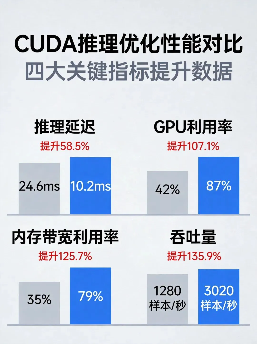
5.3 优化效果对比
图3: ResNet-50推理优化前后关键性能指标对比总结
CUDA推理优化是一个系统工程,需要深入理解硬件架构、精心设计算法、持续性能调优。本文从架构原理、内存优化、计算加速、工程实践四个维度进行了深入探讨,并通过实际案例展示了优化技术的应用效果。图4: 自动驾驶实时目标检测应用场景关键要点总结:
- 内存优化是基础
- 计算优化是核心: Tensor Core、ILP等技术可显著提升计算效率
- 工程实践是保障: 流并发、Graph优化等高级技术将理论转化为实际性能
- 性能分析是指南
随着AI技术的快速发展,CUDA编程技能将在深度学习推理领域发挥越来越重要的作用。希望本文能为读者提供实用的技术指导和启发,助力构建更高效的AI推理系统。

 10个月宝宝每天需要喝多少奶粉?
