Python 绘制“玫瑰图”:接触方向分布与接触力强度可视化(含代码)

引言

在颗粒材料、离散元模拟、岩土剪切试验和接触力链分析中，我们经常会遇到一类很典型的数据：一列是接触法向角度，另一列是对应的接触力大小。单独看这些原始数据，很难直接判断接触方向是否具有明显的优势方向，也不容易看出哪些方向上的接触力更强。为了更直观地展示这种“方向—力学量”关系，可以把 0°–360° 圆周等分成若干个角度扇区，例如每 10° 一个扇区，然后统计每个扇区内的接触数量、平均接触力、总接触力或最大接触力。最后用极坐标柱状图的方式绘制出来，就可以形成一张具有方向统计意义的玫瑰图。本文绘制两张图：第一张是接触力均值玫瑰图，第二张是接触数量与平均接触力的双层玫瑰图。前者适合展示不同方向上的接触力强弱，后者则可以同时对比“哪个方向接触更多”和“哪个方向接触更强”。

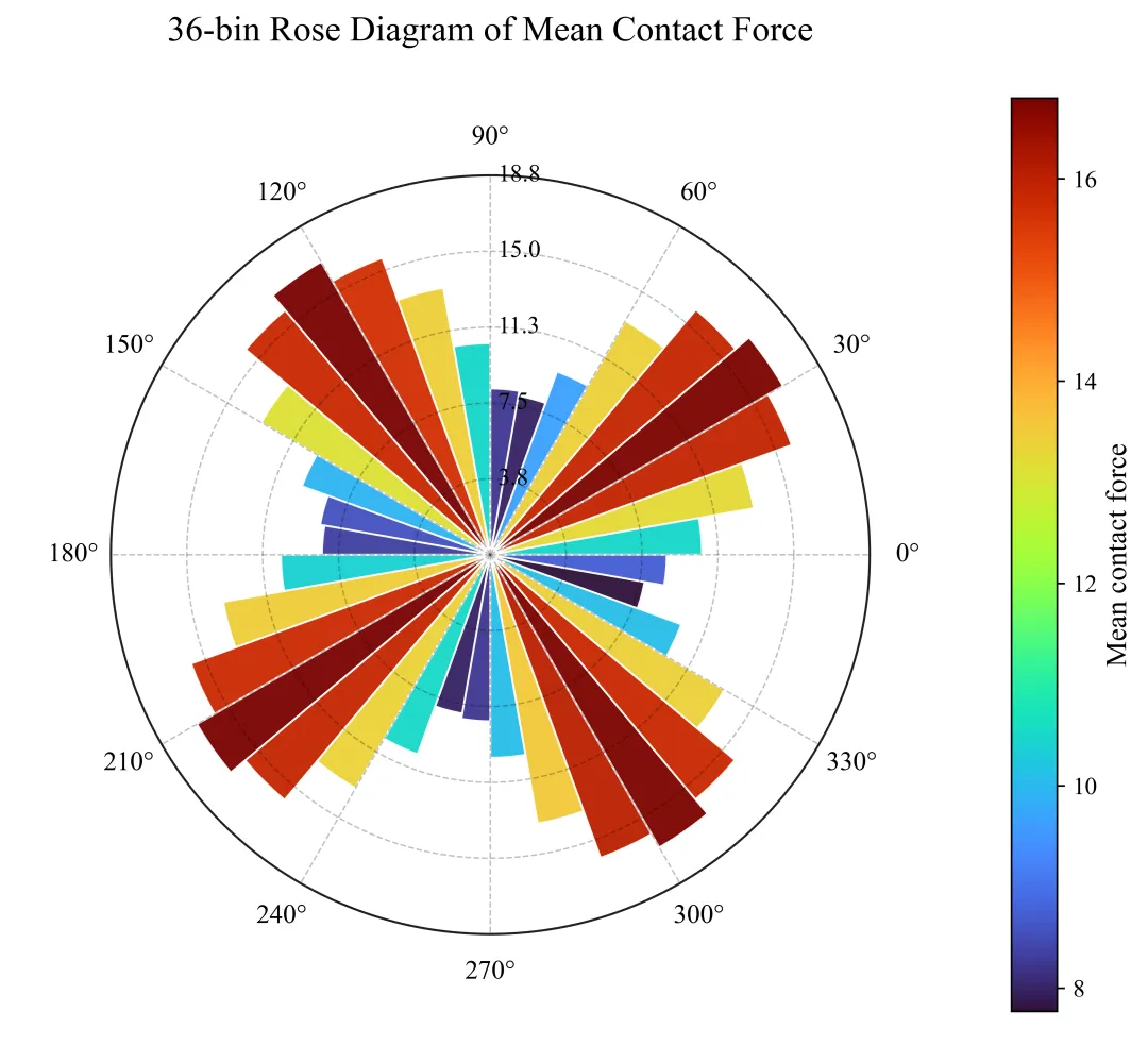
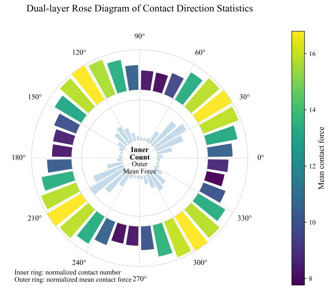
import osimport numpy as npimport matplotlib.pyplot as pltfrom matplotlib.patches import Wedgefrom matplotlib.colors import Normalizefrom matplotlib.cm import ScalarMappablenp.random.seed(2026)plt.rcParams["font.family"] = "Times New Roman"plt.rcParams["axes.unicode_minus"] = Falseplt.rcParams["figure.dpi"] = 160plt.rcParams["savefig.dpi"] = 600out_dir = "python_contact_rose_figures"os.makedirs(out_dir, exist_ok=True)def generate_contact_data(n=5000):    """    随机生成离散元接触方向数据    angle_deg      : 接触法向角度，单位 degree，范围 0~360    contact_force  : 接触力大小    """    # 设置几个主要接触方向，模拟颗粒材料中的各向异性    main_dirs = np.array([35, 125, 215, 305])    # 不同主方向出现概率不同    group = np.random.choice(        len(main_dirs),        size=n,        p=[0.34, 0.16, 0.34, 0.16]    )    # 主方向附近随机扰动    angle_deg = np.random.normal(        loc=main_dirs[group],        scale=13,        size=n    )    # 加入一部分均匀随机背景接触    n_background = int(0.20 * n)    angle_deg[:n_background] = np.random.uniform(0, 360, size=n_background)    angle_deg = np.mod(angle_deg, 360)    # 构造接触力：让接触力也随方向变化    theta = np.deg2rad(angle_deg)    force_direction_effect = (        8.0        + 4.8 * np.cos(2 * (theta - np.deg2rad(35))) ** 2        + 2.2 * np.cos(4 * (theta - np.deg2rad(35)))    )    force_random = np.random.gamma(        shape=2.2,        scale=0.85,        size=n    )    contact_force = force_direction_effect + force_random    contact_force = np.clip(contact_force, 0.2, None)    return angle_deg, contact_forceangle_deg, contact_force = generate_contact_data(n=5000)n_bins = 36edges_deg = np.linspace(0, 360, n_bins + 1)centers_deg = (edges_deg[:-1] + edges_deg[1:]) / 2mean_force = np.zeros(n_bins)sum_force = np.zeros(n_bins)max_force = np.zeros(n_bins)count_force = np.zeros(n_bins)for i in range(n_bins):    left = edges_deg[i]    right = edges_deg[i + 1]    if i < n_bins - 1:        mask = (angle_deg >= left) & (angle_deg < right)    else:        mask = (angle_deg >= left) & (angle_deg <= right)    count_force[i] = np.sum(mask)    if np.any(mask):        mean_force[i] = np.mean(contact_force[mask])        sum_force[i] = np.sum(contact_force[mask])        max_force[i] = np.max(contact_force[mask])    else:        mean_force[i] = 0        sum_force[i] = 0        max_force[i] = 0# 3. 图1：36 等分接触力均值玫瑰图def draw_mean_force_rose():    values = mean_force.copy()    color_values = mean_force.copy()    cmap = plt.get_cmap("turbo")    norm = Normalize(        vmin=np.min(color_values),        vmax=np.max(color_values)    )    rmax = np.max(values) * 1.12    if rmax <= 0:        rmax = 1    fig, ax = plt.subplots(figsize=(7.6, 7.6))    ax.set_aspect("equal")    ax.axis("off")    # 绘制36个扇形柱    for k in range(n_bins):        theta1 = edges_deg[k]        theta2 = edges_deg[k + 1]        wedge = Wedge(            center=(0, 0),            r=values[k],            theta1=theta1,            theta2=theta2,            width=values[k],            facecolor=cmap(norm(color_values[k])),            edgecolor="white",            linewidth=0.9,            alpha=0.96        )        ax.add_patch(wedge)    # 径向网格圈    theta = np.linspace(0, 2 * np.pi, 800)    ring_values = np.linspace(0, rmax, 6)[1:]    for rr in ring_values:        ax.plot(            rr * np.cos(theta),            rr * np.sin(theta),            linestyle="--",            linewidth=0.7,            color="black",            alpha=0.25        )    # 角度辐射线    angle_ticks = np.arange(0, 360, 30)    for a in angle_ticks:        ar = np.deg2rad(a)        ax.plot(            [0, rmax * np.cos(ar)],            [0, rmax * np.sin(ar)],            linestyle="--",            linewidth=0.7,            color="black",            alpha=0.25        )    # 最外圈    ax.plot(        rmax * np.cos(theta),        rmax * np.sin(theta),        color="black",        linewidth=1.0,        alpha=0.85    )    # 径向刻度文字    for rr in ring_values:        x = rr * np.cos(np.deg2rad(90))        y = rr * np.sin(np.deg2rad(90))        ax.text(            x + 0.02 * rmax,            y,            f"{rr:.1f}",            fontsize=11,            ha="left",            va="center"        )    # 角度标注    for a in angle_ticks:        ar = np.deg2rad(a)        x = rmax * 1.10 * np.cos(ar)        y = rmax * 1.10 * np.sin(ar)        ax.text(            x,            y,            f"{a}°",            fontsize=12,            ha="center",            va="center"        )    sm = ScalarMappable(norm=norm, cmap=cmap)    sm.set_array([])    cbar = fig.colorbar(        sm,        ax=ax,        shrink=0.78,        pad=0.04    )    cbar.set_label("Mean contact force", fontsize=13)    cbar.ax.tick_params(labelsize=11)    ax.set_title(        "36-bin Rose Diagram of Mean Contact Force",        fontsize=16,        pad=18    )    lim = rmax * 1.25    ax.set_xlim(-lim, lim)    ax.set_ylim(-lim, lim)    plt.tight_layout()    plt.savefig(        os.path.join(out_dir, "01_mean_contact_force_rose.png"),        bbox_inches="tight",        facecolor="white"    )draw_mean_force_rose()# 4. 图2：双层方向统计玫瑰图#    内层：接触数量#    外层：平均接触力def draw_dual_layer_rose():    count_norm = count_force / np.max(count_force)    force_norm = mean_force / np.max(mean_force)    cmap = plt.get_cmap("viridis")    norm = Normalize(        vmin=np.min(mean_force),        vmax=np.max(mean_force)    )    fig, ax = plt.subplots(figsize=(7.8, 7.8))    ax.set_aspect("equal")    ax.axis("off")    r_inner_base = 0.18    r_inner_max = 0.58    r_outer_base = 0.68    r_outer_max = 1.08    # 内层：接触数量    for k in range(n_bins):        theta1 = edges_deg[k] + 0.8        theta2 = edges_deg[k + 1] - 0.8        r = r_inner_base + count_norm[k] * (r_inner_max - r_inner_base)        wedge = Wedge(            center=(0, 0),            r=r,            theta1=theta1,            theta2=theta2,            width=r - r_inner_base,            facecolor="#BFD7EA",            edgecolor="white",            linewidth=0.8,            alpha=0.92        )        ax.add_patch(wedge)    # 外层：平均接触力    for k in range(n_bins):        theta1 = edges_deg[k] + 0.8        theta2 = edges_deg[k + 1] - 0.8        r = r_outer_base + force_norm[k] * (r_outer_max - r_outer_base)        wedge = Wedge(            center=(0, 0),            r=r,            theta1=theta1,            theta2=theta2,            width=r - r_outer_base,            facecolor=cmap(norm(mean_force[k])),            edgecolor="white",            linewidth=0.8,            alpha=0.96        )        ax.add_patch(wedge)    # 网格圈    theta = np.linspace(0, 2 * np.pi, 800)    for rr in [r_inner_base, r_inner_max, r_outer_base, r_outer_max]:        ax.plot(            rr * np.cos(theta),            rr * np.sin(theta),            linestyle="--",            linewidth=0.8,            color="black",            alpha=0.25        )    # 角度辐射线    angle_ticks = np.arange(0, 360, 30)    for a in angle_ticks:        ar = np.deg2rad(a)        ax.plot(            [0, r_outer_max * np.cos(ar)],            [0, r_outer_max * np.sin(ar)],            linestyle="--",            linewidth=0.7,            color="black",            alpha=0.22        )    # 角度标注    for a in angle_ticks:        ar = np.deg2rad(a)        x = r_outer_max * 1.12 * np.cos(ar)        y = r_outer_max * 1.12 * np.sin(ar)        ax.text(            x,            y,            f"{a}°",            fontsize=12,            ha="center",            va="center"        )    # 中心说明    ax.text(        0,        0.04,        "Inner\nCount",        fontsize=12,        ha="center",        va="center",        weight="bold"    )    ax.text(        0,        -0.10,        "Outer\nMean Force",        fontsize=11,        ha="center",        va="center"    )    # 左下角说明    ax.text(        -1.25,        -1.18,        "Inner ring: normalized contact number\nOuter ring: normalized mean contact force",        fontsize=11,        ha="left",        va="center"    )    sm = ScalarMappable(norm=norm, cmap=cmap)    sm.set_array([])    cbar = fig.colorbar(        sm,        ax=ax,        shrink=0.75,        pad=0.05    )    cbar.set_label("Mean contact force", fontsize=13)    cbar.ax.tick_params(labelsize=11)    ax.set_title(        "Dual-layer Rose Diagram of Contact Direction Statistics",        fontsize=16,        pad=18    )    lim = 1.35    ax.set_xlim(-lim, lim)    ax.set_ylim(-lim, lim)    plt.tight_layout()    plt.savefig(        os.path.join(out_dir, "02_dual_layer_contact_rose.png"),        bbox_inches="tight",        facecolor="white"    )draw_dual_layer_rose()

特别声明：

以上代码与文案均为网上资料整合而成，仅供广大同行们参考学习，如有侵权请联系删除。