“ 提供定制化绘图服务,支持先出样图,满意后付款,私信联系我们。”
之前有许多朋友不知道如何获取完整的代码与数据,在这里分享给大家完整的步骤,了解的朋友请跳过,直接阅读正文:
1、点击关注:
完毕。
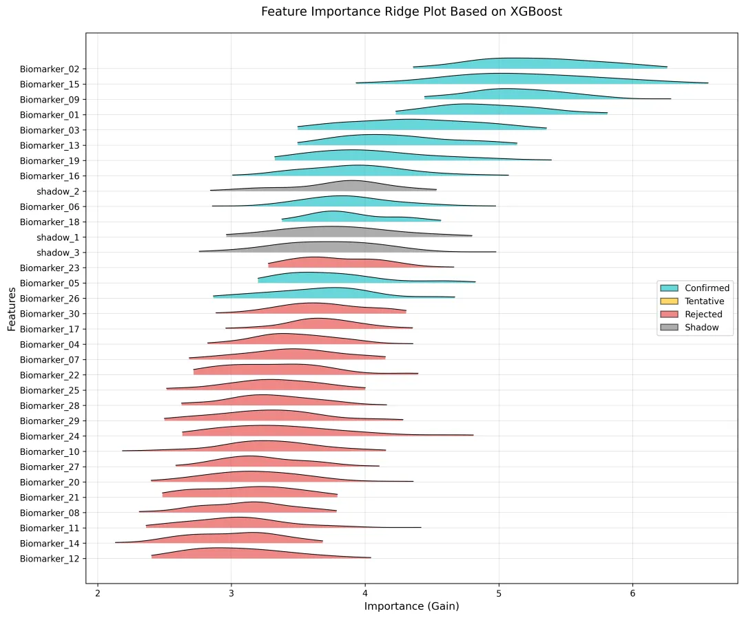
代码以 XGBoost 算法为例,通过多随机种子训练模型获取特征增益型重要性,引入影子特征作参照并按分位数将特征分类,再经核密度估计拟合重要性分布,最终绘制山脊图可视化特征重要性差异。实现过程为先生成或读取模拟数据,自动识别特征与目标列,多轮训练提取并处理重要性数据,完成特征分类后转换数据格式,基于核密度估计绘制并保存可视化山脊图,实现特征重要性的量化与可视化分析。
模块导入与绘图参数配置段
导入数据分析与绘图库,屏蔽警告并配置 Matplotlib 全局绘图参数;原理是调用 Python 库功能,通过 rcParams 修改绘图全局属性;实现为 import 导入库,warnings 过滤警告,设置字体、dpi 等参数。
import osimport warningsimport numpy as npimport pandas as pdimport xgboost as xgbimport matplotlib.pyplot as pltfrom scipy.stats import gaussian_kdewarnings.filterwarnings('ignore')plt.rcParams['font.sans-serif'] = ['DejaVu Sans']plt.rcParams['axes.unicode_minus'] = Falseplt.rcParams['figure.dpi'] = 300plt.rcParams['savefig.dpi'] = 300plt.rcParams['figure.figsize'] = (12, 10)
数据文件读写逻辑
功能为判断数据文件是否存在,实现模拟数据生成保存或已有数据读取;原理是通过 os 模块判断文件路径存在性,pandas 实现 Excel 文件的读写;实现是 os.path.exists 判断路径,调用模拟函数并通过 to_excel/read_excel 处理文件。
file_path = "data(山脊图).xlsx"if not os.path.exists(file_path): clinical_dataset = simulate_clinical_data(num_patients=500, num_biomarkers=30) clinical_dataset.to_excel(file_path, index=False) print("已生成模拟数据并保存到文件")else: clinical_dataset = pd.read_excel(file_path) print(f"已从文件读取数据,数据形状: {clinical_dataset.shape}") print(f"列名: {list(clinical_dataset.columns)}")
目标列与特征列自动识别函数
功能为自动匹配目标列并分离特征列,无预定义列则默认最后一列为目标列;原理是遍历预定义目标列候选名,匹配成功则分离,无匹配则取最后一列;实现是循环候选名,列表推导式筛选特征列,打印识别结果。
def auto_detect_columns(data): target_candidates = ['outcome', 'target', 'label', 'y', 'class', 'diagnosis', 'response'] for candidate in target_candidates: if candidate in data.columns: target_col = candidate feature_cols = [col for col in data.columns if col != target_col] print(f"自动识别目标列为: '{target_col}'") print(f"特征数量: {len(feature_cols)}") return target_col, feature_cols print("警告: 未找到预定义的目标列名称") print("请从以下列中选择目标列:") for i, col in enumerate(data.columns): print(f"{i}: {col}") target_col = data.columns[-1] feature_cols = [col for col in data.columns if col != target_col] print(f"默认使用最后一列作为目标列: '{target_col}'") print(f"特征数量: {len(feature_cols)}") return target_col, feature_cols
列识别函数调用
功能为执行列识别函数,获取数据集的目标列和特征列变量;原理是调用已定义的自动列识别函数,传入数据集作为参数;实现是直接调用 auto_detect_columns,接收函数返回的目标列和特征列结果。
target_col, feature_cols = auto_detect_columns(clinical_dataset)
功能为多随机种子训练 XGB 模型,获取特征重要性历史数据并生成影子特征;原理是多轮训练降低随机误差,提取增益型重要性,生成正态分布影子特征作参照;实现是循环训练 XGB 分类器,get_score 提取重要性,numpy 生成影子列数据。
def get_xgb_feature_importance(data, target_col=target_col, feature_cols=feature_cols, n_iter=50): X = data[feature_cols] y = data[target_col] print(f"使用目标列: {target_col}") print(f"使用特征列: {feature_cols}") imp_history = [] random_seeds = [250307 + i for i in range(n_iter)] for seed in random_seeds: model = xgb.XGBClassifier(objective='binary:logistic', random_state=seed, n_estimators=100, max_depth=3, learning_rate=0.1, subsample=0.8, colsample_bytree=0.8, n_jobs=-1) model.fit(X, y) imp = model.get_booster().get_score(importance_type='gain') imp_full = {feat: imp.get(feat, 0.0) for feat in feature_cols} imp_history.append(imp_full) imp_history_df = pd.DataFrame(imp_history) for i in range(3): shadow_col = f"shadow_{i + 1}" imp_history_df[shadow_col] = np.random.normal(loc=imp_history_df[feature_cols].mean().mean(), scale=imp_history_df[feature_cols].std().mean(), size=n_iter) return imp_history_df
特征重要性函数调用
功能为执行 XGBoost 特征重要性计算,获取含影子特征的重要性历史数据;原理是调用已定义的重要性计算函数,传入数据集及列参数;实现是调用 get_xgb_feature_importance,接收返回的重要性历史 DataFrame。
imp_history = get_xgb_feature_importance(clinical_dataset, target_col, feature_cols, n_iter=50)
特征分类函数
功能为依据影子特征分位数将真实特征分三类,合并影子特征形成完整分类表;原理是计算影子特征 95 分位数均值,对比真实特征分位数判定类别;实现是 quantile 计算分位数,条件判断分类,pandas 拼接真实与影子特征数据。
def classify_features(imp_history, feature_cols): shadow_cols = [col for col in imp_history.columns if 'shadow' in col] real_cols = feature_cols shadow_95 = imp_history[shadow_cols].quantile(0.95, axis=0).mean() feature_decisions = [] for feat in real_cols: feat_95 = imp_history[feat].quantile(0.95) if feat_95 > shadow_95: decision = "Confirmed" elif imp_history[feat].quantile(0.75) > shadow_95: decision = "Tentative" else: decision = "Rejected" feature_decisions.append(decision) real_decision = pd.DataFrame({'feature': real_cols, 'decision': feature_decisions}) shadow_decision = pd.DataFrame({'feature': shadow_cols, 'decision': ["Shadow"] * len(shadow_cols)}) all_decision = pd.concat([real_decision, shadow_decision], ignore_index=True) return all_decision
特征分类统计打印
功能为输出不同类别特征的数量统计结果;原理是利用 pandas 的 value_counts 方法统计分类列的频次分布;实现是调用 decision_all ['decision'].value_counts () 并打印统计结果。
decision_all = classify_features(imp_history, feature_cols)print("\n特征分类统计:")print(decision_all['decision'].value_counts())
数据格式转换与预处理
功能为将重要性数据宽转长,合并分类结果并过滤缺失值,确定特征排序;原理是 melt 实现宽格式转长格式,merge 合并分类信息,按中位数排序特征;实现是调用 melt、merge,通过 np.isfinite 过滤缺失值,groupby 计算中位数并排序。
imp_history_long = imp_history.melt(var_name='feature', value_name='importance')imp_history_long = imp_history_long.merge(decision_all, on='feature', how='left')imp_history_long_clean = imp_history_long[np.isfinite(imp_history_long['importance'])].copy()feature_order = imp_history_long_clean.groupby('feature')['importance'].median().sort_values().index.tolist()
山脊图绘制函数
功能为基于特征重要性分布绘制山脊图并保存图像;原理是用核密度估计拟合重要性数据分布,偏移绘制各特征的密度曲线;实现是 gaussian_kde 拟合分布,fill_between 填充曲线区域,设置坐标轴并保存图像。
def plot_ridgeplot(data, feature_order, color_scheme, save_path): fig, ax = plt.subplots(figsize=(12, 10)) scale = 0.8 y_offsets = {feat: i * scale for i, feat in enumerate(feature_order)} for feat in feature_order: feat_data = data[data['feature'] == feat]['importance'] kde = gaussian_kde(feat_data) x_vals = np.linspace(feat_data.min(), feat_data.max(), 500) y_vals = kde(x_vals) y_vals = y_vals / y_vals.max() * scale * 0.7 y_base = y_offsets[feat] decision = data[data['feature'] == feat]['decision'].iloc[0] color = color_scheme.get(decision, (0.8, 0.8, 0.8, 0.6)) ax.fill_between(x_vals, y_base, y_base + y_vals, color=color[:3], alpha=color[3], edgecolor=None, linewidth=0) ax.plot(x_vals, y_base + y_vals, color='black', linewidth=0.8, linestyle='-') ax.grid(True, color='gray', alpha=0.3, linestyle='-', linewidth=0.5) ax.set_yticks([y_offsets[feat] for feat in feature_order]) ax.set_yticklabels(feature_order, fontsize=10) ax.set_xlabel('Importance (Gain)', fontsize=12) ax.set_ylabel('Features', fontsize=12) ax.set_title('Feature Importance Ridge Plot Based on XGBoost', fontsize=14, pad=20) legend_elements = [plt.Rectangle((0, 0), 1, 1, facecolor=color[:3], alpha=color[3], edgecolor='black', label=dec) for dec, color in color_scheme.items()] ax.legend(handles=legend_elements, loc='right', frameon=True, fontsize=10) plt.tight_layout() plt.savefig(save_path, bbox_inches='tight', dpi=300) plt.close()
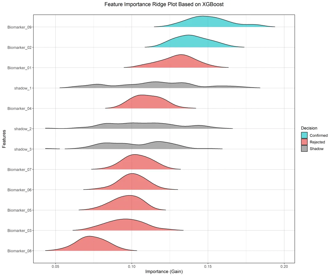
R语言这里就不再分段解释,完整附上代码及效果图:
library(rstudioapi)setwd(dirname(rstudioapi::getSourceEditorContext()$path))library(readxl)library(xgboost)library(dplyr)library(tidyr)library(ggplot2)library(ggridges)library(scales)library(parallel)library(tibble) # 加载tibble包,提供rownames_to_column函数options(warn=-1)file_path <- "data(山脊图).xlsx"if (!file.exists(file_path)) { stop("文件不存在,请先生成数据")} else { clinical_dataset <- read_excel(file_path) cat(sprintf("已从文件读取数据,数据形状: %d x %d\n", nrow(clinical_dataset), ncol(clinical_dataset))) cat(sprintf("列名: %s\n", paste(colnames(clinical_dataset), collapse=", ")))}auto_detect_columns <- function(data) { target_candidates <- c('outcome', 'target', 'label', 'y', 'class', 'diagnosis', 'response') for (candidate in target_candidates) { if (candidate %in% colnames(data)) { target_col <- candidate feature_cols <- colnames(data)[colnames(data) != target_col] cat(sprintf("自动识别目标列为: '%s'\n", target_col)) cat(sprintf("特征数量: %d\n", length(feature_cols))) return(list(target_col = target_col, feature_cols = feature_cols)) } } cat("警告: 未找到预定义的目标列名称\n") cat("请从以下列中选择目标列:\n") for (i in seq_along(colnames(data))) { cat(sprintf("%d: %s\n", i-1, colnames(data)[i])) } target_col <- colnames(data)[length(colnames(data))] feature_cols <- colnames(data)[colnames(data) != target_col] cat(sprintf("默认使用最后一列作为目标列: '%s'\n", target_col)) cat(sprintf("特征数量: %d\n", length(feature_cols))) return(list(target_col = target_col, feature_cols = feature_cols))}detect_result <- auto_detect_columns(clinical_dataset)target_col <- detect_result$target_colfeature_cols <- detect_result$feature_colsget_xgb_feature_importance <- function(data, target_col, feature_cols, n_iter=50) { X <- as.matrix(data[, feature_cols]) y <- as.numeric(data[, target_col][[1]]) cat(sprintf("使用目标列: %s\n", target_col)) cat(sprintf("使用特征列: %s\n", paste(feature_cols, collapse=", "))) imp_history <- list() random_seeds <- 250307 + 0:(n_iter-1) for (seed in random_seeds) { params <- list( objective = "binary:logistic", seed = seed, max_depth = 3, eta = 0.1, subsample = 0.8, colsample_bytree = 0.8, nthread = detectCores() ) dtrain <- xgb.DMatrix(data = X, label = y) model <- xgb.train( params = params, data = dtrain, nrounds = 100, verbose = 0 ) # 核心修正:移除R中不存在的importance_type参数 imp <- xgb.importance(feature_names = feature_cols, model = model) imp_df <- as.data.frame(imp) imp_full <- setNames(rep(0, length(feature_cols)), feature_cols) imp_full[imp_df$Feature] <- imp_df$Gain imp_history[[as.character(seed)]] <- imp_full } imp_history_df <- do.call(rbind, imp_history) %>% as.data.frame() for (i in 1:3) { shadow_col <- sprintf("shadow_%d", i) mean_val <- mean(unlist(imp_history_df[, feature_cols])) std_val <- sd(unlist(imp_history_df[, feature_cols])) imp_history_df[[shadow_col]] <- rnorm(n_iter, mean = mean_val, sd = std_val) } return(imp_history_df)}imp_history <- get_xgb_feature_importance(clinical_dataset, target_col, feature_cols, n_iter=50)classify_features <- function(imp_history, feature_cols) { shadow_cols <- colnames(imp_history)[grepl("shadow", colnames(imp_history))] real_cols <- feature_cols shadow_95 <- mean(apply(imp_history[, shadow_cols], 2, quantile, 0.95)) feature_decisions <- sapply(real_cols, function(feat) { feat_95 <- quantile(imp_history[[feat]], 0.95) if (feat_95 > shadow_95) { "Confirmed" } else if (quantile(imp_history[[feat]], 0.75) > shadow_95) { "Tentative" } else { "Rejected" } }) real_decision <- data.frame( feature = real_cols, decision = feature_decisions, stringsAsFactors = FALSE ) shadow_decision <- data.frame( feature = shadow_cols, decision = rep("Shadow", length(shadow_cols)), stringsAsFactors = FALSE ) all_decision <- rbind(real_decision, shadow_decision) return(all_decision)}decision_all <- classify_features(imp_history, feature_cols)cat("\n特征分类统计:\n")print(table(decision_all$decision))# 修正后:加载tibble包后可正常使用rownames_to_columnimp_history_long <- imp_history %>% rownames_to_column("seed") %>% pivot_longer(cols = -seed, names_to = "feature", values_to = "importance") %>% left_join(decision_all, by = "feature") %>% filter(is.finite(importance))feature_order <- imp_history_long %>% group_by(feature) %>% summarise(median_importance = median(importance), .groups = "drop") %>% arrange(median_importance) %>% pull(feature)imp_history_long$feature <- factor(imp_history_long$feature, levels = feature_order)original_colors <- c( "Confirmed" = rgb(0.0078, 0.7373, 0.7569, 0.6), "Tentative" = rgb(1.0, 0.7569, 0.0275, 0.6), "Rejected" = rgb(0.8980, 0.2235, 0.2078, 0.6), "Shadow" = rgb(0.4588, 0.4588, 0.4588, 0.6))plot_ridgeplot <- function(data, feature_order, color_scheme, save_path) { ggplot(data, aes(x = importance, y = feature, fill = decision)) + geom_density_ridges( scale = 0.8, alpha = 0.6, size = 0.8, color = "black", rel_min_height = 0.01, from = min(imp_history_long$importance) ) + scale_fill_manual(values = color_scheme, drop = FALSE) + theme_bw() + theme( text = element_text(family = "DejaVu Sans"), axis.text = element_text(size = 10), axis.title = element_text(size = 12), plot.title = element_text(size = 14, margin = margin(b = 20), hjust = 0.5), legend.position = "right", legend.text = element_text(size = 10), panel.grid = element_line(color = "gray", alpha = 0.1, linewidth = 0.3) ) + labs( x = "Importance (Gain)", y = "Features", title = "Feature Importance Ridge Plot Based on XGBoost", fill = "Decision" ) + coord_cartesian(clip = "off") ggsave( filename = save_path, width = 12, height = 10, dpi = 300, bg = "white", device = "png", limitsize = FALSE )}plot_ridgeplot( data = imp_history_long, feature_order = feature_order, color_scheme = original_colors, save_path = "xgboost_ridgeplot_original.png")cat(sprintf("\n山脊图已保存为: xgboost_ridgeplot_original.png\n"))
私信我“260128”,免费获取完整python/R语言代码和示例数据。