期刊图片复现|Python绘制多模型对比二分类任务ROC曲线
- 2026-10-11 07:19:36
期刊图片复现|Python绘制多模型对比二分类任务ROC曲线

论文:TCellSI: A novel method for T cell state assessment and its applications in immune environment prediction 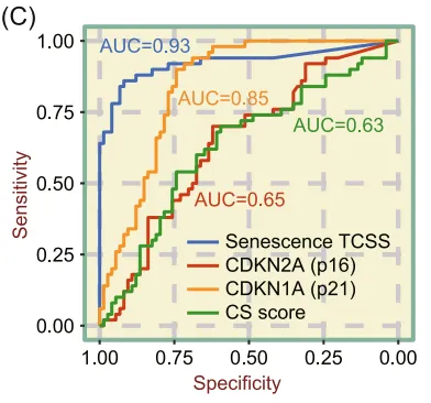
论文原图 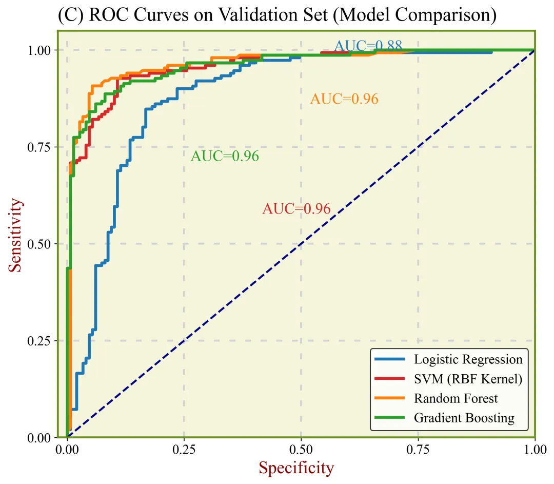
仿图 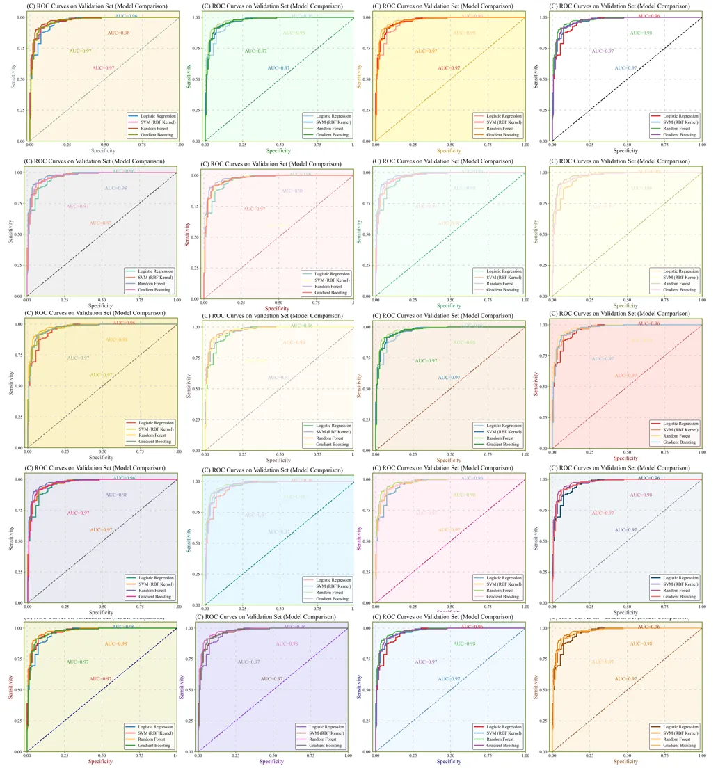
多种配色 



库的导入以及字体设置 

颜色库的设置以及配色方案的选择 

绘图函数 接受真实标签、一个包含所有模型预测分数的字典、图表标题、颜色字典和保存的文件名等参数,这里面要记得修改函数末尾部分的保存路径,还有要记得调整一下那几个文本标注的位置 

数据的加载与处理部分 包括原始数据的读取、特征数据和标签的分离、训练数据和验证数据的划分、标准化处理等,这里记得修改数据的输入地址、特征数据和目标的列的等 

模型构建 训练了4个模型,包括逻辑回归模型、支持向量机模型、随机森林模型、GBT模型,这里要记得修改模型的超参数,因为我现在都是瞎设置的,你一定要根据自己的任务目标来进行一下重新设定 

调用函数进行绘图 



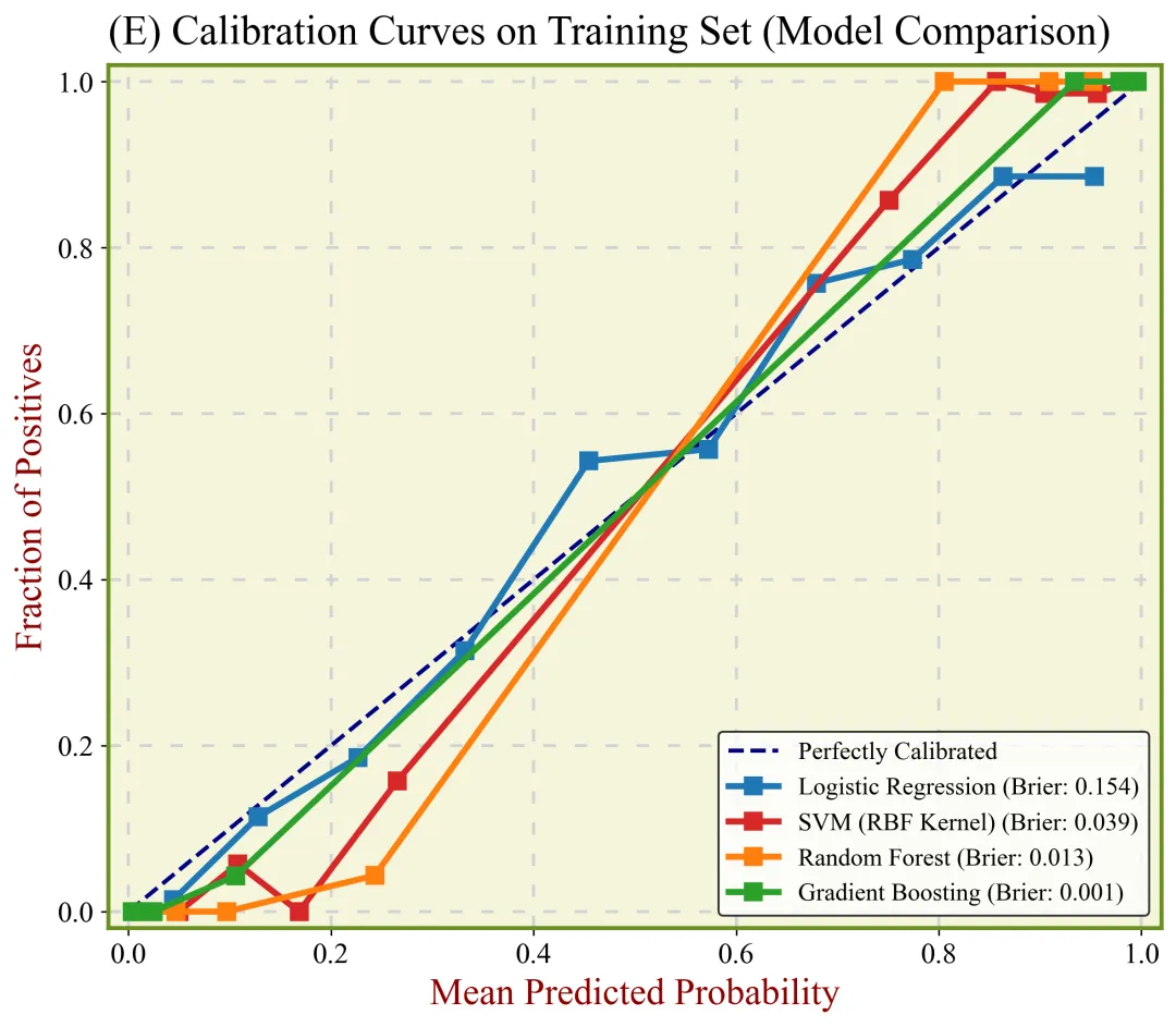
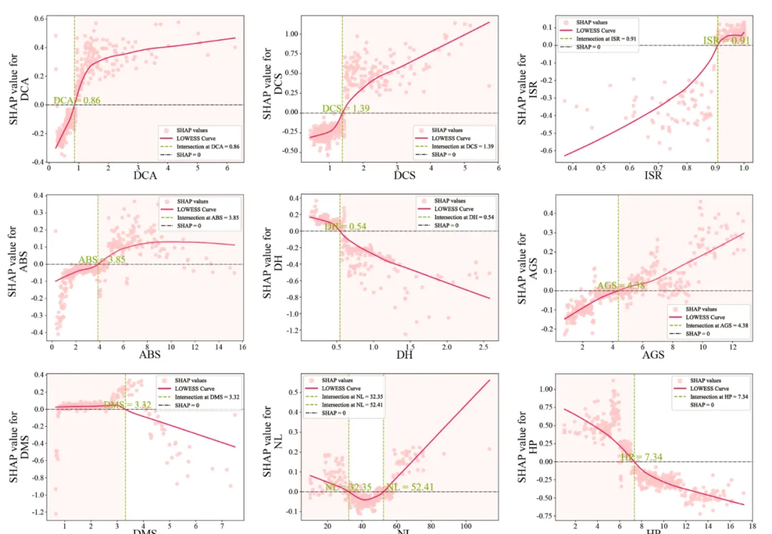
期刊图片复现|Python绘制二维偏依赖PDP图 期刊复现|python绘制基于SHAP分析和GAM模型拟合的单特征依赖图 期刊图片复现|python绘制带有渐变颜色shap特征重要性组合图(条形图+蜂巢图) 期刊复现|用Python绘制SHAP特征重要性总览图、依赖图、双特征交互效应SHAP图,解锁XGBoost模型的终极奥秘 期刊图片复现|Python绘制shap重要性蜂巢图+单特征依赖图+交互效应强度气泡图+交互效应依赖图(回归+二分类+分类) 



需要的请后台私信我获取详细信息,注意只会分享练习数据和代码文件,不会提供答疑服务,代码文件中已经包含了每行代码的完整注释!!!
代码绘制成果展示
代码解释
第一部分
import pandas as pdimport matplotlib.pyplot as pltfrom sklearn.model_selection import train_test_split, GridSearchCVfrom sklearn.preprocessing import StandardScalerfrom sklearn.linear_model import LogisticRegressionfrom sklearn.svm import SVCfrom sklearn.ensemble import RandomForestClassifier, GradientBoostingClassifierfrom sklearn.metrics import roc_curve, aucimport sysplt.rcParams['font.family'] = 'serif'plt.rcParams['font.serif'] = ['Times New Roman']plt.rcParams['axes.unicode_minus'] = Falseimport matplotlibmatplotlib.rcParams['pdf.fonttype'] = 42matplotlib.rcParams['ps.fonttype'] = 42
第二部分
color_schemes= {1: {"Logistic Regression": '#1f77b4', "SVM (RBF Kernel)": '#d62728', "Random Forest": '#ff7f0e', "Gradient Boosting": '#2ca02c',"diag_line": 'navy', "xy_label": '#8B0000', "bg_color": '#F5F5DC'},}selected_scheme= 2 #选择颜色方案SELECTED_COLORS = color_schemes[selected_scheme]#获取颜色方案
第三部分
def plot_roc_curves(y_true, all_scores, plot_title, colors_dict,filename=None):fig, ax = plt.subplots(figsize=(8, 7)) #画布ax.set_facecolor(colors_dict['bg_color']) # 设置的背景颜色# 网格线ax.grid(True,which='both',linestyle='--',linewidth=2,color='lightgrey',dashes=(3, 5))#存储每个模型AUC值的文本标注位置auc_text_positions = {"Logistic Regression": (0.65, 0.95),"Random Forest": (0.6, 0.82),"Gradient Boosting": (0.35, 0.68),"SVM (RBF Kernel)": (0.5, 0.55)}#绘制对角虚线/参考线ax.plot([0, 1], [0, 1], color=colors_dict['diag_line'], lw=2, linestyle='--')ax.set_xlim([-0.02, 1.0]) #设置X轴的范围ax.set_ylim([0, 1.05]) #设置Y轴的范围ax.set_xlabel('Specificity', fontsize=18, color=colors_dict['xy_label']) #x轴标题ax.set_ylabel('Sensitivity', fontsize=18, color=colors_dict['xy_label']) #Y轴标题ax.set_title(plot_title, fontsize=20, loc='left', pad=10) #设置主图标题ax.xaxis.set_major_locator(plt.MultipleLocator(0.25)) #设置X轴主刻度的间隔ax.yaxis.set_major_locator(plt.MultipleLocator(0.25)) #设置Y轴主刻度的间隔ax.tick_params(axis='both', which='major', labelsize=14) #主刻度标签的字体大小# 添加图例ax.legend(loc='lower right', fontsize=14, frameon=True, edgecolor='black')#遍历图框for spine in ax.spines.values():spine.set_edgecolor('#6B8E23') #颜色spine.set_linewidth(2) #图框的粗细设置plt.tight_layout() # 自动调整子图参数,使其填充整个图窗区域,防止标签重叠
第四部分
excel_filename = r'data.xlsx'#原始数据路径df = pd.read_excel(excel_filename, engine='openpyxl')#读取数据# 提取所有特征和标签y = df.iloc[:, 0].valuesX= df.iloc[:, 1:].values#划分数据集为训练集和验证集X_train, X_val, y_train, y_val = train_test_split(X, y,test_size=0.3,random_state=42,stratify=y)#标准化处理scaler = StandardScaler()X_train_scaled = scaler.fit_transform(X_train)X_val_scaled = scaler.transform(X_val)
第五部分
print(f"正在为 'Logistic Regression' 进行网格搜索")#初始化逻辑回归模型model_lr = LogisticRegression(random_state=42, solver='liblinear')#逻辑回归的超参数搜索网格param_grid_lr = {'C': [0.01, 0.1, 1, 10, 100],'penalty': ['l1', 'l2']}#配置网格搜索grid_search_lr = GridSearchCV(estimator=model_lr, param_grid=param_grid_lr, cv=5, scoring='roc_auc', n_jobs=-1, verbose=0)#执行网格搜索grid_search_lr.fit(X_train_scaled, y_train)best_model_lr = grid_search_lr.best_estimator_ #最佳模型print(f"'Logistic Regression' 网格搜索完成!最佳超参数: {grid_search_lr.best_params_}")#最佳逻辑回归模型预测正类的概率scores_lr_train = best_model_lr.predict_proba(X_train_scaled)[:, 1]scores_lr_val = best_model_lr.predict_proba(X_val_scaled)[:, 1]print(f"\n--- 正在为 'SVM (RBF Kernel)' 进行网格搜索")#初始化SVC模型model_svm = SVC(random_state=42, probability=True)#超参数搜索网格param_grid_svm = {'C': [0.1, 1, 10],'gamma': [0.01, 0.1, 1]}#网格搜索grid_search_svm = GridSearchCV(estimator=model_svm, param_grid=param_grid_svm, cv=5, scoring='roc_auc', n_jobs=-1, verbose=0)grid_search_svm.fit(X_train_scaled, y_train)#最佳SVM模型best_model_svm = grid_search_svm.best_estimator_print(f"SVM最佳超参数: {grid_search_svm.best_params_}")#预测正类的概率scores_svm_train = best_model_svm.predict_proba(X_train_scaled)[:, 1]scores_svm_val = best_model_svm.predict_proba(X_val_scaled)[:, 1]print(f"\n--- 正在为 'Random Forest' 进行网格搜索")#初始化RF模型model_rf = RandomForestClassifier(random_state=42)#超参数搜索网格param_grid_rf = {'n_estimators': [50, 100, 200],'max_depth': [5, 10, None]}#执行网格搜索grid_search_rf = GridSearchCV(estimator=model_rf, param_grid=param_grid_rf, cv=5, scoring='roc_auc', n_jobs=-1, verbose=0)grid_search_rf.fit(X_train_scaled, y_train)#最佳RF模型best_model_rf = grid_search_rf.best_estimator_print(f"'RF最佳超参数: {grid_search_rf.best_params_}")#预测正类的概率scores_rf_train = best_model_rf.predict_proba(X_train_scaled)[:, 1]scores_rf_val = best_model_rf.predict_proba(X_val_scaled)[:, 1]print(f"\n--- 正在为 'Gradient Boosting' 进行网格搜索 ---")# 初始化GBT模型model_gbt = GradientBoostingClassifier(random_state=42)param_grid_gbt = {'n_estimators': [50, 100],'learning_rate': [0.05, 0.1],'max_depth': [3, 5]}#执行网格搜索grid_search_gbt = GridSearchCV(estimator=model_gbt, param_grid=param_grid_gbt, cv=5, scoring='roc_auc', n_jobs=-1, verbose=0)grid_search_gbt.fit(X_train_scaled, y_train)#最佳GBT模型best_model_gbt = grid_search_gbt.best_estimator_print(f"GBT最佳超参数: {grid_search_gbt.best_params_}")#预测正类的概率scores_gbt_train = best_model_gbt.predict_proba(X_train_scaled)[:, 1]scores_gbt_val = best_model_gbt.predict_proba(X_val_scaled)[:, 1]
第六部分
#存储训练集上所有模型的预测分数train_scores_dict = {"Logistic Regression": scores_lr_train,"SVM (RBF Kernel)": scores_svm_train,"Random Forest": scores_rf_train,"Gradient Boosting": scores_gbt_train}#存储验证集上所有模型的预测分数val_scores_dict = {"Logistic Regression": scores_lr_val,"SVM (RBF Kernel)": scores_svm_val,"Random Forest": scores_rf_val,"Gradient Boosting": scores_gbt_val}#绘制训练集的ROC曲线plot_roc_curves(y_train,train_scores_dict,"(C) ROC Curves on Training Set (Model Comparison)",SELECTED_COLORS,filename='train')#绘制验证集的ROC曲线plot_roc_curves(y_val,val_scores_dict,"(C) ROC Curves on Validation Set (Model Comparison)",SELECTED_COLORS,filename='test')
如何应用?
1.选择你想要使用到的配色方案:
selected_scheme= 20 #选择颜色方案2.修改图面的文本标注位置:
auc_text_positions = {"Logistic Regression": (0.65, 0.95),"Random Forest": (0.6, 0.82),"Gradient Boosting": (0.35, 0.68),"SVM (RBF Kernel)": (0.5, 0.55)}
3.设置绘图结果的保存路径:
fig.savefig(fr'{filename}_{selected_scheme}.png', dpi=300, bbox_inches='tight')fig.savefig(fr'{filename}_{selected_scheme}.pdf', bbox_inches='tight')
4.设置原始数据的输入路径位置:
excel_filename = r'simulated_senescence_data.xlsx'#原始数据路径5.设置数据划分:
y = df.iloc[:, 0].valuesX= df.iloc[:, 1:].values
6.修改各个模型的超参数:
param_grid_lr = { 'C': [0.01, 0.1, 1, 10, 100], 'penalty': ['l1', 'l2']}推荐
预告
获取方式
本文来自网友投稿或网络内容,如有侵犯您的权益请联系我们删除,联系邮箱:596563534@qq.com 。
